Introduction to Mechanics for Engineersby Andy Ruina & Rudra Pratap0 What is mechanics?2 Free-Body Diagrams

Chapter 1 Vectors for mechanics: position, force and moment

Download this chapter by section

1.0Introductionstudy PDF
1.1Notation and additionstudy PDF + solutions
1.2The dot product of two vectorsstudy PDF + solutions
1.3Vector cross productstudy PDF + solutions
1.4Momentstudy PDF + solutions
1.5Solving vector equationsstudy PDF + solutions

Mechanical analysis uses vectors. We develop vector skills here using the key vectors for statics, namely relative position, force, and moment. Notational clarity is emphasized because good vector calculation demands distinguishing vectors from scalars. Vector addition is motivated by the need to add forces and relative positions. Dot products are motivated as the tool which reduces vector equations to scalar equations. And cross products are motivated as the formula which correctly calculates the heuristically-motivated quantities of moment and moment about an axis.

In these books you will learn to use the laws of mechanics which were informally introduced in Chapter 1. This means calculating with mechanics-relevant quantities. The most fundamental quantities in mechanics are the two scalars,

•

mass $m$ and
•

time $t$ ,

and the two vectors,

•

relative position ${\accentset{\rightharpoonup}{\boldsymbol{r}}}_{i\mathrm{/O}}$ (position of point $i$ relative to point O), and
•

force ${\accentset{\rightharpoonup}{\boldsymbol{F}}}$ (acting on a system of interest) ^†^†margin: Actually, one can argue that ${\accentset{\rightharpoonup}{\boldsymbol{F}}}$ isn’t fundamental because it can be defined in terms of $m$ and ${\accentset{\rightharpoonup}{\boldsymbol{a}}}$ which, in turn, are defined in terms of ${\accentset{\rightharpoonup}{\boldsymbol{r}}}$ and $t$ . But, both historically and in most engineering practice, ${\accentset{\rightharpoonup}{\boldsymbol{F}}}$ is treated as a fundamental quantity.

Scalars are typed with an italic font ( $t$ and $m$ ) and vectors are typed in bold with a harpoon on top ( ${\accentset{\rightharpoonup}{\boldsymbol{r}}}_{i\mathrm{/O}}$ , ${\accentset{\rightharpoonup}{\boldsymbol{F}}}$ ). All the other scalars (see box 1.1 on page 1.1) and vectors (see box 1.1 on page 1.1) that we use in mechanics are defined in terms of $m,t,{\accentset{\rightharpoonup}{\boldsymbol{r}}}_{i\mathrm{/O}}$ and ${\accentset{\rightharpoonup}{\boldsymbol{F}}}$ . If you are a legitimate reader of this book, you are already good at scalar arithmetic and algebra (adding, subtracting, multiplying and dividing ordinary numbers and symbols representing numbers). For mechanics you also need facility with the vector arithmetic and algebra, as explained in this chapter.

Filename:tfigure8-rel-ang-vel

Figure 1.1: Vector

{\accentset{\rightharpoonup}{\boldsymbol{A}}}

2\,\mathrm{cm}

long and points Northeast. Two copies of

{\accentset{\rightharpoonup}{\boldsymbol{A}}}

are drawn to show that where the drawing is placed doesn’t affect the vector. It’s the same vector drawn in two different places.

What is a vector?

Whereas a scalar is just a (possibly dimensional

^†^†margin: By ‘dimensional’ we mean ‘with units’ like meters, Newtons, or kg. (We don’t mean: having an abstract vector-space dimension, as in one, two or three dimensional.

), single number, a thing with magnitude and a sign,

a vector is a (possibly dimensional) quantity that is fully described by both magnitude and direction.

Example: NorthEast 2 cm

As a first vector example, consider a line segment with a length (magnitude) of $2\,\mathrm{cm}$ . The segment has a tail end and a head end. It is pointed Northeast. Let’s call this vector ${\accentset{\rightharpoonup}{\boldsymbol{A}}}$ (see fig. 1.1).

{\accentset{\rightharpoonup}{\boldsymbol{A}}}\mathrel{\mathop{=}\limits^{def}}% \mbox{$2\,\mathrm{cm}$ long line segment pointed Northeast}

In terms of our basic list at the top of the page, ${\accentset{\rightharpoonup}{\boldsymbol{A}}}$ is the relative position ${\accentset{\rightharpoonup}{\boldsymbol{r}}}_{h/t}$ of its head $h$ relative to its tail $t$ .

Every vector in mechanics is well visualized as an arrow. The direction of the arrow is the direction of the vector. The length of the arrow is proportional to the magnitude of the vector. The magnitude of ${\accentset{\rightharpoonup}{\boldsymbol{A}}}$ is a positive scalar indicated by $|{\accentset{\rightharpoonup}{\boldsymbol{A}}}|$ . A vector does not lose its identity if it is picked up and moved around in space (so long as it is not rotated nor stretched). Thus, both vectors drawn in fig. 1.1 are the same vector ${\accentset{\rightharpoonup}{\boldsymbol{A}}}$ .

Vector arithmetic makes sense

We have oversimplified. We said that a vector is something with magnitude and direction. In fact, by common modern convention, that’s not enough. A one way street sign, for example, is not considered a vector even though it has a magnitude (its mass is, say, half a kilogram) and a direction (the direction that most of the traffic goes). We need more to call something a vector. A thing is only called a vector if, additionally, elementary vector arithmetic, vector addition in particular, has a sensible meaning

^†^†margin: In abstract mathematics they don’t bother to talk about magnitudes and directions. All they care about is vector arithmetic. So, to the mathematicians, anything which obeys simple vector arithmetic is a vector, arrow-like or not. In math talk, lots of strange things are vectors, like arrays of numbers and functions. As special cases of the mathematicians’ ‘abstract vectors’, the vectors in this book always have magnitude and direction.

The following sentence summarizes centuries of thought and also motivates this chapter:

The vectors in mechanics have magnitude and direction and elementary vector arithmetic operations have sensible physical meanings.

This chapter is about vector arithmetic. In this chapter you will learn how to add and subtract vectors, how to stretch them, how to find their components, and how to multiply them with each other two different ways. Each of these operations has use in mechanics.

1.1 Vector notation and vector addition

Facility with vectors has several aspects.

1.

You must recognize which quantities are vectors (such as relative position) and which are scalars (such as length).
2.

You have to use a notation that distinguishes between vectors and scalars using, for example, ${\accentset{\rightharpoonup}{\boldsymbol{a}}}$ , or $\underline{\boldsymbol{a}}$ for acceleration and $a$ for a scalar with the same magnitude so that $|a|=|{\accentset{\rightharpoonup}{\boldsymbol{a}}}|$ .
3.

You need skills in vector arithmetic, perhaps more than you learned in your previous math and physics courses.

In this first section (1.1) we start with notation. Mastery of the notation, perhaps a seemingly petty topic, is surprisingly well-correlated with mastery of mechanics. We go on to find the relative position vector from a picture, to multiplication of a vector by a scalar, and to vector addition and vector subtraction.

How to write vectors

A scalar is written as a single English or Greek letter. This book uses italics for scalars (e.g., $m$ for mass) but ordinary printing is fine for hand work (e.g., m for mass). A vector is also represented by a single letter of the alphabet, either English or Greek, but ornamented to indicate that it is a vector and not a scalar. The common ornamentations are described below.

Use one of these vector notations in all of your work

^†^†margin: Be careful to distinguish vectors from scalars in all of your written work. Clear notation helps clear thinking and will help you solve problems. If you notice that you are not using clear vector notation, stop, determine which quantities are vectors and which scalars, and fix your notation. Rare is the student who consistently gets correct answers to exam questions without clear vector notation. And almost as rare is the student who has clear vector usage and can’t do problems. For some students, accepting this vector language and syntax is a bitter pill. Just swallow it. You’ll feel much better.

Box 1.1 The scalars in mechanics

Most of the scalars in this book are listed below. Dimensions (units) are given in brackets [ ], ( $M$ for mass, $L$ for length, $T$ for time, $F$ for force, and $E$ for energy).

•

mass $m$ , [ $M$ ];
•

length or distance $\ell$ , $w$ , $x$ , $r$ , $\rho$ , $d$ , or $s$ , [ $L$ ];
•

time $t$ , [ $T$ ];
•

pressure $p$ , [ $F/L^{2}]=[M/(L\cdot T^{2})$ ];
•

angles $\theta$ ‘theta’, $\phi$ ‘phi’, $\gamma$ ‘gamma’, and $\psi$ ‘psi’, [dimensionless];
•

energy $E$ , kinetic energy ${E_{\mathrm{K}}}$ , potential energy ${E_{\mathrm{P}}}$ , [ $E$ ] $=$ [ $F\cdot L$ ] $=$ [ $M\cdot L^{2}/T^{2}$ ];
•

work $W$ , [ $E$ ] $=$ [ $F\cdot L$ ] $=$ [ $M\cdot L^{2}/T^{2}$ ];
•

tension $T$ , [ $M\cdot L/T^{2}$ ] $=$ [ $F$ ];
•

power $P$ , [ $E/T$ ] $=$ [ $M\cdot L^{2}/T^{3}$ ];
•
the magnitudes of all the vector quantities are also scalars, for example
- –
  
  speed $|{\accentset{\rightharpoonup}{\boldsymbol{v}}}|$ , [ $L/T$ ];
- –
  
  magnitude of acceleration $|{\accentset{\rightharpoonup}{\boldsymbol{a}}}|$ , [ $L/T^{2}$ ];
- –
  
  magnitude of angular momentum $|{\accentset{\rightharpoonup}{\boldsymbol{H}}}|$ , [ $M\cdot L^{2}/T$ ];
•
the components of vectors, for example
- –
  
  $r_{x}\quad$ (where ${\accentset{\rightharpoonup}{\boldsymbol{r}}}=r_{x}\hat{\boldsymbol{\imath}}+r% _{y}\hat{\boldsymbol{\jmath}}$ ), or
- –
  
  $L_{x^{\prime}}\quad$ (where ${\accentset{\rightharpoonup}{\boldsymbol{L}}}=L_{x^{\prime}}\hat{\boldsymbol{% \imath}}^{\prime}+L_{y^{\prime}}\hat{\boldsymbol{\jmath}}^{\prime}$ );
•

coefficient of friction $\mu$ ‘mu’, or friction angle $\phi$ ‘phi’;
•

coefficient of restitution $e$ ;
•

mass per unit length, area, or volume $\rho$ ;
•

oscillation frequency $\beta$ or $\lambda$ .

Box 1.2 The Vectors in Mechanics

The vector quantities used in mechanics, and the notations for them used in this book, are shown below. The dimensional symbols of each are shown in brackets [ ].

•

position ${\accentset{\rightharpoonup}{\boldsymbol{r}}}$ or ${\accentset{\rightharpoonup}{\boldsymbol{x}}}$ , [ $L$ ];
•

velocity ${\accentset{\rightharpoonup}{\boldsymbol{v}}}$ or $\dot{\accentset{\rightharpoonup}{\boldsymbol{x}}}$ or $\dot{\accentset{\rightharpoonup}{\boldsymbol{r}}}$ , [ $L/T$ ];
•

acceleration ${\accentset{\rightharpoonup}{\boldsymbol{a}}}$ or $\dot{\accentset{\rightharpoonup}{\boldsymbol{v}}}$ or $\ddot{\accentset{\rightharpoonup}{\boldsymbol{r}}}$ , [ $L/T^{2}$ ];
•

angular velocity ${\accentset{\rightharpoonup}{\boldsymbol{\omega}}}$ ‘omega’ (or, if aligned with the $\hat{\boldsymbol{k}}$ axis, $\dot{\theta}{\hat{\boldsymbol{k}}}$ ), [ $1/T$ ];
•

rate of change of angular velocity ${\accentset{\rightharpoonup}{\boldsymbol{\alpha}}}$ ‘alpha’ or $\dot{\accentset{\rightharpoonup}{\boldsymbol{\omega}}}$ (or, if aligned with the $\hat{\boldsymbol{k}}$ axis, $\ddot{\theta}\hat{\boldsymbol{k}}$ ), [ $1/T^{2}$ ];
•

force ${\accentset{\rightharpoonup}{\boldsymbol{F}}}$ or ${\accentset{\rightharpoonup}{\boldsymbol{N}}}$ , [ $m\cdot L/T^{2}$ ] $=$ [ $F$ ];
•

moment or torque ${\accentset{\rightharpoonup}{\boldsymbol{M}}}$ , [ $m\cdot L^{2}/T^{2}$ ] $=$ [ $F\cdot L$ ];
•

linear momentum ${\accentset{\rightharpoonup}{\boldsymbol{L}}}$ , [ $m\cdot L/T$ ] and its rate of change $\dot{\accentset{\rightharpoonup}{\boldsymbol{L}}}$ , [ $m\cdot L/T^{2}$ ];
•

angular momentum ${\accentset{\rightharpoonup}{\boldsymbol{H}}}$ , [ $m\cdot L^{2}/T$ ]; and its rate of change $\dot{\accentset{\rightharpoonup}{\boldsymbol{H}}}$ , [ $m\cdot L^{2}/T^{2}$ ].
•
unit vectors to help write other vectors [dimensionless]:
- –
  
  $\hat{\boldsymbol{\imath}}$ , $\hat{\boldsymbol{\jmath}}$ , and $\hat{\boldsymbol{k}}$ for cartesian coordinates,
- –
  
  $\hat{\boldsymbol{\imath}}^{\prime}$ , $\hat{\boldsymbol{\jmath}}^{\prime}$ , and $\hat{\boldsymbol{k}}^{\prime}$ for crooked cartesian coordinates,
- –
  
  $\hat{\boldsymbol{e}}_{r}$ and $\hat{\boldsymbol{e}}_{\scriptscriptstyle\!\theta}$ for polar coordinates,
- –
  
  $\hat{\boldsymbol{e}}_{t}$ and $\hat{\boldsymbol{e}}_{n}$ for path coordinates, and
- –
  
  $\hat{\boldsymbol{\lambda}}$ ‘lambda’ and $\hat{\boldsymbol{n}}$ as miscellaneous unit vectors.

Ornamentation of vectors. Subscripts and superscripts are often added to indicate the point, points, object, or objects the vectors are describing. Upper case letters (O, A, B, C,…) are used to denote points. Upper case calligraphic (or script if you are writing by hand) letters ( $\cal A,B,C...F...$ ) are for labeling rigid objects or reference frames. $\cal F$ , or $\cal N$ , is the fixed, Newtonian, or ‘absolute’ reference frame (think of $\cal F$ as the ground if you are a first-time reader). For example, ${\accentset{\rightharpoonup}{\boldsymbol{r}}}_{\!\mathrm{AB}}$ or ${\accentset{\rightharpoonup}{\boldsymbol{r}}}_{\!\mathrm{B/A}}$ is the position of the point $B$ relative to point $A$ . ${\accentset{\rightharpoonup}{\boldsymbol{\omega}}}_{\cal B}$ is the absolute angular velocity of the object called $\cal B$ ( ${\accentset{\rightharpoonup}{\boldsymbol{\omega}}}_{\cal B}$ is short hand for ${\accentset{\rightharpoonup}{\boldsymbol{\omega}}}_{\cal B/F}$ ). And ${\accentset{\rightharpoonup}{\boldsymbol{H}}}_{{\cal A}/C}$ is the angular momentum of object $\cal A$ relative to point $C$ (We will explain the meaning of the words ‘angular velocity’ and ‘angular momentum’ in the dynamics book. Here, we are just using them to show the subscript ornamentation. ).

The notation is further complicated when we want to take derivatives with respect to moving frames, a topic which comes up later in the Dynamics book. For completeness here: ${}^{\cal B}\dot{\accentset{\rightharpoonup}{\boldsymbol{\omega}}}_{\cal D/E}$ is the time derivative with respect to reference frame $\cal B$ of the angular velocity of object $\cal D$ with respect to object (or frame) $\cal E$ . (If this paragraph doesn’t read like gibberish to you, you have already studied dynamics. This paragraph is for the experts who are looking back.)

${\accentset{\rightharpoonup}{\boldsymbol{F}}}$: Putting a harpoon (or arrow) over the letter $\boldsymbol{F}$ . The arrow is suggestive of the idea of a vector. This is the notation used in this book.
$\boldsymbol{F}$: In most texts a bold $\boldsymbol{F}$ represents the vector ${\accentset{\rightharpoonup}{\boldsymbol{F}}}$ . But, bold face is inconvenient for hand written work. The lack of bold face pens and pencils tempts students to transcribe a bold $\boldsymbol{F}$ as $F$ . But $F$ with no adornment represents a scalar and not a vector. So, when using other books, take care to transcribe $\boldsymbol{F}$ as ${\accentset{\rightharpoonup}{\boldsymbol{F}}}$ or as $\underline{F}$ .
$\underline{\boldsymbol{F}}$: Underlining or under-squiggling ( $\hbox to0.0pt{\boldsymbol{F}\hss}_{{}_{\sim}}$ ) is an easy and unambiguous notation for hand writing vectors. A recent Gallup poll survey found that 117 out of 168 mechanics professors use this notation. These professors would copy a ${\accentset{\rightharpoonup}{\boldsymbol{F}}}$ from this book by writing $\underline{F}$ . The origin of the underline notation seems to be from typesetting. In the pre-computer days, a book author would indicate that a letter should be printed in bold by underlining it.
$\bar{\boldsymbol{F}}$: It is a stroke simpler to put a bar rather than a harpoon over a symbol. But the saved effort causes ambiguity. Why? An over-bar is often used to indicate average. There could then be confusion, say, between the velocity $\bar{v}$ and the average speed $\bar{v}$ .
$\hat{\boldsymbol{\imath}}$: Over-hat. Putting a hat on top is like an over-arrow or over-bar. In this book we reserve the hat for unit vectors. For example, we use $\hat{\boldsymbol{\imath}}$ , $\hat{\boldsymbol{\jmath}}$ , and $\hat{\boldsymbol{k}}$ , or $\hat{\boldsymbol{e}}_{1}$ , $\hat{\boldsymbol{e}}_{2}$ , and $\hat{\boldsymbol{e}}_{3}$ for unit vectors parallel to the $x$ , $y$ , and $z$ axes, respectively. The same poll of 168 mechanics professors found that 32 of them used no special notation for unit vectors and just wrote them like, e.g., $\underline{\boldsymbol{\imath}}$ .

Drawing vectors

In fig. 1.1 on page 1.1, the magnitude of ${\accentset{\rightharpoonup}{\boldsymbol{A}}}$ was represented by the drawing length. But drawing a vector using its magnitude as length would be awkward if, say, we were interested in vector ${\accentset{\rightharpoonup}{\boldsymbol{B}}}$ that points Northwest and has a magnitude of $2\,\mbox{meters}$ . To fit ${\accentset{\rightharpoonup}{\boldsymbol{B}}}$ in a drawing would require a piece of paper about 2 meters square (each edge the length of a basketball player). This situation moves from difficult to ridiculous if the magnitude of the vector of interest is $2\,{\mbox{km}}$ and it would take half an hour to draw the vector by walking from tail to tip dragging a purple crayon. Thus, in pictures, we merely make scale drawings of vectors with, for example, one centimeter of graph paper representing 1 kilometer of vector magnitude.

Filename:tfigure8-ang-vel-ex

Figure 1.2: Position and force vectors are drawn with different scales.

The necessity for using scale drawings to represent vectors is especially apparent for a vector whose magnitude is not length. Force is a vector since it has magnitude and direction. Say ${\accentset{\rightharpoonup}{\boldsymbol{F}}}_{\rm gr}$ is the $700\,{\mbox{N}}$ force that the ground pushes up on your chair as you sit reading. We can’t draw a line segment with length $700\,{\mbox{N}}$ for ${\accentset{\rightharpoonup}{\boldsymbol{F}}}_{\rm gr}$ because a Newton is a unit of force not a unit of length. So, a scale drawing is the only choice.

One often needs to draw vectors with different units on the same picture, as for showing the position ${\accentset{\rightharpoonup}{\boldsymbol{r}}}$ at which a force ${\accentset{\rightharpoonup}{\boldsymbol{F}}}$ is applied (see fig. 1.2). In this case, even though the vectors are on the same drawing, different scale factors are used for the drawing of the vectors that have different units.

Drawing and measuring are tedious, and also not very accurate. And drawing in 3 dimensions is particularly hard (given the poor quality of 3D graph paper nowadays). So, the magnitudes and directions of vectors are usually defined with numbers and units rather than scale drawings. Despite that we will ultimately calculate using numbers and lists of numbers, the drawing rules and geometric descriptions define all the vector concepts.

Adding vectors

Tip to tail rule. The sum of two vectors ${\accentset{\rightharpoonup}{\boldsymbol{A}}}$ and ${\accentset{\rightharpoonup}{\boldsymbol{B}}}$ is defined by the tip to tail rule of vector addition shown in fig. 1.3a for the sum ${\accentset{\rightharpoonup}{\boldsymbol{C}}}={\accentset{\rightharpoonup}{% \boldsymbol{A}}}+{\accentset{\rightharpoonup}{\boldsymbol{B}}}$ . Vector ${\accentset{\rightharpoonup}{\boldsymbol{A}}}$ is drawn. Then, vector ${\accentset{\rightharpoonup}{\boldsymbol{B}}}$ is drawn with its tail at the tip (or head) of ${\accentset{\rightharpoonup}{\boldsymbol{A}}}$ . The sum ${\accentset{\rightharpoonup}{\boldsymbol{C}}}$ is the vector from the tail of ${\accentset{\rightharpoonup}{\boldsymbol{A}}}$ to the tip of ${\accentset{\rightharpoonup}{\boldsymbol{B}}}$ .

Parallelogram rule. The same sum is achieved if ${\accentset{\rightharpoonup}{\boldsymbol{B}}}$ is drawn first, as shown in fig. 1.3b. Putting both ways of adding ${\accentset{\rightharpoonup}{\boldsymbol{A}}}$ and ${\accentset{\rightharpoonup}{\boldsymbol{B}}}$ on the same picture draws a parallelogram as shown in fig. 1.3c. Hence the tip to tail rule of vector addition is also called the parallelogram rule. The parallelogram construction shows the commutative property of vector addition, namely that ${\accentset{\rightharpoonup}{\boldsymbol{A}}}+{\accentset{\rightharpoonup}{% \boldsymbol{B}}}={\accentset{\rightharpoonup}{\boldsymbol{B}}}+{\accentset{% \rightharpoonup}{\boldsymbol{A}}}$ .

3D. Note that you can view fig. 1.3a-c as 3D pictures. In 3D, the parallelogram will be on a plane but that may well be tilted relative to the $x, y$ and $z$ axes.

Filename:tfigure8-ang-vel

Figure 1.3: (a) tip to tail addition of

{\accentset{\rightharpoonup}{\boldsymbol{A}}}+{\accentset{\rightharpoonup}{% \boldsymbol{B}}}

, (b) tip to tail addition of

{\accentset{\rightharpoonup}{\boldsymbol{B}}}+{\accentset{\rightharpoonup}{% \boldsymbol{A}}}

, (c) the parallelogram interpretation of vector addition which shows the commutative law of vector addition:

{\accentset{\rightharpoonup}{\boldsymbol{A}}}+{\accentset{\rightharpoonup}{% \boldsymbol{B}}}={\accentset{\rightharpoonup}{\boldsymbol{B}}}+{\accentset{% \rightharpoonup}{\boldsymbol{A}}}

, and (d) The associative law of vector addition:

({\accentset{\rightharpoonup}{\boldsymbol{A}}}+{\accentset{\rightharpoonup}{% \boldsymbol{B}}})+{\accentset{\rightharpoonup}{\boldsymbol{D}}}={\accentset{% \rightharpoonup}{\boldsymbol{A}}}+({\accentset{\rightharpoonup}{\boldsymbol{B}% }}+{\accentset{\rightharpoonup}{\boldsymbol{D}}})

.

This figure also makes sense in 3D. Drawings (a), (b) and (c) are all on a tilted planes. And the 6 vectors drawn in (d) lie on the edges of a tetrahedron.

Adding many vectors. Three vectors are added by the same tip to tail rule. The construction shown in fig. 1.3d shows that $({\accentset{\rightharpoonup}{\boldsymbol{A}}}+{\accentset{\rightharpoonup}{% \boldsymbol{B}}})+{\accentset{\rightharpoonup}{\boldsymbol{D}}}={\accentset{% \rightharpoonup}{\boldsymbol{A}}}+({\accentset{\rightharpoonup}{\boldsymbol{B}% }}+{\accentset{\rightharpoonup}{\boldsymbol{D}}})$ so that the expression ${\accentset{\rightharpoonup}{\boldsymbol{A}}}+{\accentset{\rightharpoonup}{% \boldsymbol{B}}}+{\accentset{\rightharpoonup}{\boldsymbol{D}}}$ is unambiguous. This is the associative property of vector addition. Showing this triple sum in all different orders and groupings draws a parallelepiped (with some extra lines). Thus, one might call the geometric addition of three vectors in 3D the ‘parallelepiped rule’ for vector addition (but no-one does).

With these two properties, the commutative and associative laws of vector addition, we see that the sum ${\accentset{\rightharpoonup}{\boldsymbol{A}}}+{\accentset{\rightharpoonup}{% \boldsymbol{B}}}+{\accentset{\rightharpoonup}{\boldsymbol{D}}}+\dots$ can be permuted to ${\accentset{\rightharpoonup}{\boldsymbol{D}}}+{\accentset{\rightharpoonup}{% \boldsymbol{A}}}+{\accentset{\rightharpoonup}{\boldsymbol{B}}}+\dots$ , or any which way, without changing the result. That is, vector addition shares the associativity and commutativity of scalar addition that you are used to e.g., that $3+(7+\pi)=(\pi+3)+7$ .

Concurrent forces. We can reconsider the statement ‘force is a vector’ and see that it hides (or contains) one of the basic assumptions in mechanics, namely:

If forces ${\accentset{\rightharpoonup}{\boldsymbol{F}}}_{\!\!\mathrm{1}}$ and ${\accentset{\rightharpoonup}{\boldsymbol{F}}}_{\!\!\mathrm{2}}$ are applied to a point on a structure they can be replaced, for all mechanics considerations, with a single force ${\accentset{\rightharpoonup}{\boldsymbol{F}}}={\accentset{\rightharpoonup}{% \boldsymbol{F}}}_{\!\!\mathrm{1}}+{\accentset{\rightharpoonup}{\boldsymbol{F}}% }_{\!\!\mathrm{2}}$ applied to that point

as illustrated in fig. 1.4. The force ${\accentset{\rightharpoonup}{\boldsymbol{F}}}$ is said to be equivalent to the concurrent (acting at one point) force system consisting of ${\accentset{\rightharpoonup}{\boldsymbol{F}}}_{\!\!\mathrm{1}}$ and ${\accentset{\rightharpoonup}{\boldsymbol{F}}}_{\!\!\mathrm{2}}$ acting at the same point.

Filename:tfigure8-ang-accel

Figure 1.4: Two forces acting at a point may be replaced by their sum for all mechanics purposes.

Apples and oranges. Note that two vectors with different dimensions cannot be added. Figure 1.2 on page 1.2 can no more sensibly be taken to represent meaningful vector addition than can the scalar sum of a length and a weight, “ $2\,\mbox{ft}+3\,{\mbox{N}}$ ”, be taken as meaningful.

Subtraction, negation, and the zero vector

Subtraction is most simply defined by inverse addition. The expression ${\accentset{\rightharpoonup}{\boldsymbol{C}}}-{\accentset{\rightharpoonup}{% \boldsymbol{A}}}$ means: find the vector which, when added to ${\accentset{\rightharpoonup}{\boldsymbol{A}}}$ , gives ${\accentset{\rightharpoonup}{\boldsymbol{C}}}$ ^†^†margin: Just like for money. $100 - $70 means ‘find how much money you have to add to $70 to get $100’. .

We can draw ${\accentset{\rightharpoonup}{\boldsymbol{C}}}$ , draw ${\accentset{\rightharpoonup}{\boldsymbol{A}}}$ and then find the vector which, when added tip to tail to ${\accentset{\rightharpoonup}{\boldsymbol{A}}}$ , gives ${\accentset{\rightharpoonup}{\boldsymbol{C}}}$ . Figure 1.3a shows that ${\accentset{\rightharpoonup}{\boldsymbol{B}}}$ answers the question. Another interpretation comes from defining the negative of a vector $-{\accentset{\rightharpoonup}{\boldsymbol{A}}}$ as ${\accentset{\rightharpoonup}{\boldsymbol{A}}}$ with the head and tail switched. Again you can see from fig. 1.3b by imagining that the head and tail on ${\accentset{\rightharpoonup}{\boldsymbol{A}}}$ were switched to make $-{\accentset{\rightharpoonup}{\boldsymbol{A}}}$ , that ${\accentset{\rightharpoonup}{\boldsymbol{C}}}+(-{\accentset{\rightharpoonup}{% \boldsymbol{A}}})={\accentset{\rightharpoonup}{\boldsymbol{B}}}$ . The negative of a vector evidently has the expected property that ${\accentset{\rightharpoonup}{\boldsymbol{A}}}+(-{\accentset{\rightharpoonup}{% \boldsymbol{A}}})={\accentset{\rightharpoonup}{\boldsymbol{0}}}$ , where ${\accentset{\rightharpoonup}{\boldsymbol{0}}}$ is the vector with no magnitude so that ${\accentset{\rightharpoonup}{\boldsymbol{C}}}+{\accentset{\rightharpoonup}{% \boldsymbol{0}}}={\accentset{\rightharpoonup}{\boldsymbol{C}}}$ for all vectors ${\accentset{\rightharpoonup}{\boldsymbol{C}}}$ .

Relative-position vectors

The concept of relative position is used in most mechanics equations. The position of point B relative to point A is represented by the vector

{\accentset{\rightharpoonup}{\boldsymbol{r}}}_{\!\mathrm{B/A}}\ \textrm{(% pronounced `r of B relative to A')}

drawn from A and to B (as shown in fig. 1.5). An alternate notation for the relative position vector ${\accentset{\rightharpoonup}{\boldsymbol{r}}}_{\!\mathrm{B/A}}$ is

{\accentset{\rightharpoonup}{\boldsymbol{r}}}_{B/A}\equiv{\accentset{% \rightharpoonup}{\boldsymbol{r}}}_{\!\mathrm{AB}}\ \textrm{(pronounced `r A B'% or `r from A to B')}.

You can think of the position of B relative to A as being the position of B relative to you if you were standing on A. Similarly ${\accentset{\rightharpoonup}{\boldsymbol{r}}}_{\!\mathrm{C/B}}={\accentset{% \rightharpoonup}{\boldsymbol{r}}}_{\!\mathrm{BC}}$ is the position of C relative to B.

Figure 1.5a shows that relative positions add by the tip to tail rule. That is,

Filename:tfigure8-ang-accel-ex

Figure 1.5: a) Relative position of points A, B, and C; b) Relative position of points O, A, and B.

{\accentset{\rightharpoonup}{\boldsymbol{r}}}_{\!\mathrm{C/A}}={\accentset{% \rightharpoonup}{\boldsymbol{r}}}_{\!\mathrm{B/A}}+{\accentset{\rightharpoonup% }{\boldsymbol{r}}}_{\!\mathrm{C/B}}\qquad\mbox{or}\qquad{\accentset{% \rightharpoonup}{\boldsymbol{r}}}_{\!\mathrm{AC}}={\accentset{\rightharpoonup}% {\boldsymbol{r}}}_{\!\mathrm{AB}}+{\accentset{\rightharpoonup}{\boldsymbol{r}}% }_{\!\mathrm{BC}}

so, as needed to get the description ‘vector’, for relative-position vectors, vector addition has a sensible meaning.

Note that the position of B relative to A is the opposite (negative vector) of the position of A relative to B, so

{\accentset{\rightharpoonup}{\boldsymbol{r}}}_{\!\mathrm{B/A}}=-{\accentset{% \rightharpoonup}{\boldsymbol{r}}}_{\!\mathrm{A/B}}\qquad\mbox{or}\qquad{% \accentset{\rightharpoonup}{\boldsymbol{r}}}_{\!\mathrm{AB}}=-{\accentset{% \rightharpoonup}{\boldsymbol{r}}}_{\!\mathrm{BA}}.

Position relative to the origin. Often when doing problems we pick a distinguished point in space, say a prominent point or corner of a machine or structure, and use it as the origin of a coordinate system O. The position of point A relative to O is ${\accentset{\rightharpoonup}{\boldsymbol{r}}}_{\!\mathrm{A/0}}$ or ${\accentset{\rightharpoonup}{\boldsymbol{r}}}_{\!\mathrm{OA}}$ but we often adopt the shorthand notation ${\accentset{\rightharpoonup}{\boldsymbol{r}}}_{\!\mathrm{A}}$ (pronounced ‘r A’) leaving the reference point O as implied,

{\accentset{\rightharpoonup}{\boldsymbol{r}}}_{\!\mathrm{A}}\quad\textrm{means% }\quad{\accentset{\rightharpoonup}{\boldsymbol{r}}}_{\!\mathrm{A/0}}.

Figure 1.5b shows that

{\accentset{\rightharpoonup}{\boldsymbol{r}}}_{\!\mathrm{B/A}}={\accentset{% \rightharpoonup}{\boldsymbol{r}}}_{\!\mathrm{B}}-{\accentset{\rightharpoonup}{% \boldsymbol{r}}}_{\!\mathrm{A}}

which rolls off the tongue more easily than ${\accentset{\rightharpoonup}{\boldsymbol{r}}}_{\!\mathrm{B/A}}={\accentset{% \rightharpoonup}{\boldsymbol{r}}}_{\!\mathrm{B/0}}-{\accentset{\rightharpoonup% }{\boldsymbol{r}}}_{\!\mathrm{A/0}}$ , and also makes the concept of relative position easier to remember.

^†^†margin: Until we get to rotating reference frames (in the Dynamics book), you can just interpret ‘relative to’ to mean ‘minus’, as in english. ‘How much money does Rudra have relative to Andy?’ means what is Rudra’s wealth minus Andy’s wealth? What is the position of B relative to A? It is the position of B minus the position of A.

Multiplication by a scalar stretches a vector

Naturally enough $2{\accentset{\rightharpoonup}{\boldsymbol{F}}}$ means ${\accentset{\rightharpoonup}{\boldsymbol{F}}}+{\accentset{\rightharpoonup}{% \boldsymbol{F}}}$ (see fig. 1.6) and $127{\accentset{\rightharpoonup}{\boldsymbol{A}}}$ means 127 copies of ${\accentset{\rightharpoonup}{\boldsymbol{A}}}$ added up. . Similarly ${\accentset{\rightharpoonup}{\boldsymbol{A}}}/7$ or $\frac{1}{7}{\accentset{\rightharpoonup}{\boldsymbol{A}}}$ means a vector in the direction of ${\accentset{\rightharpoonup}{\boldsymbol{A}}}$ that when added to 6 copies of itself gives ${\accentset{\rightharpoonup}{\boldsymbol{A}}}$ . By combining these two ideas we can define any rational multiple of ${\accentset{\rightharpoonup}{\boldsymbol{A}}}$ . For example $\frac{29}{13}{\accentset{\rightharpoonup}{\boldsymbol{A}}}$ means add 29 copies of that vector which, when 13 copies of itself are added up gives ${\accentset{\rightharpoonup}{\boldsymbol{A}}}$ ^†^†margin: It is a mathematical fine point to extend the definition to $c{\accentset{\rightharpoonup}{\boldsymbol{A}}}$ for $c$ that is irrational (i.e., pick a sequence of rational numbers that approach $c$ in the limit). .

Combining our abilities to negate a vector and multiply it by a positive scalar, we define $-17{\accentset{\rightharpoonup}{\boldsymbol{A}}}$ as $17(-{\accentset{\rightharpoonup}{\boldsymbol{A}}})$ .

Filename:tfigure8-ang-accel1

Figure 1.6: Multiplying a vector by a scalar stretches it.

In general, for any scalar $c$ we define $c{\accentset{\rightharpoonup}{\boldsymbol{A}}}$ as the vector that is in the same direction as ${\accentset{\rightharpoonup}{\boldsymbol{A}}}$ , or opposite if $c$ is negative, and whose magnitude is multiplied by $|c|$ . Five times a $5\,{\mbox{N}}$ force pointed NorthEast is a $25\,{\mbox{N}}$ force pointed NorthEast. Minus 5 times a $5\,{\mbox{N}}$ force pointed NorthEast is a $25\,{\mbox{N}}$ force pointed SouthWest.

Distributive rule for scalar multiplication of vectors. If you imagine stretching a whole vector addition diagram (e.g., fig. 1.3a on page 1.3) equally in all directions the distributive rule for scalar multiplication is apparent. Here’s what happens when you multiply the sum of the vectors $v A$ and ${\accentset{\rightharpoonup}{\boldsymbol{B}}}$ by the scalar $c$ :

c({\accentset{\rightharpoonup}{\boldsymbol{A}}}+{\accentset{\rightharpoonup}{% \boldsymbol{B}}})=c{\accentset{\rightharpoonup}{\boldsymbol{A}}}+c{\accentset{% \rightharpoonup}{\boldsymbol{B}}},

the scalar multiplication ‘distributes’.

Unit vectors have magnitude = 1

Unit vectors are vectors with a magnitude of one. Unit vectors are useful for indicating direction. Key examples are the unit vectors pointed in the positive $x, y$ and $z$ directions $\hat{\boldsymbol{\imath}}$ (called ‘i hat’ or just ‘i’), $\hat{\boldsymbol{\jmath}}$ , and $\hat{\boldsymbol{k}}$ . These three unit vectors are also called $\hat{\boldsymbol{e}}_{x},\hat{\boldsymbol{e}}_{y}$ , and $\hat{\boldsymbol{e}}_{z}$ , or $\hat{\boldsymbol{e}}_{1},\hat{\boldsymbol{e}}_{2}$ , and $\hat{\boldsymbol{e}}_{3}$ .

An easy way to find a unit vector in the direction of a vector ${\accentset{\rightharpoonup}{\boldsymbol{A}}}$ is to divide ${\accentset{\rightharpoonup}{\boldsymbol{A}}}$ by its magnitude. Thus

\hat{\boldsymbol{\lambda}}_{A}\equiv\frac{{\accentset{\rightharpoonup}{% \boldsymbol{A}}}}{|{\accentset{\rightharpoonup}{\boldsymbol{A}}}|}

is a unit vector in the ${\accentset{\rightharpoonup}{\boldsymbol{A}}}$ direction. We can check that this defines a unit vector by checking the rules for multiplication by a scalar: multiplying ${\accentset{\rightharpoonup}{\boldsymbol{A}}}$ by the scalar ${1}/{|{\accentset{\rightharpoonup}{\boldsymbol{A}}}|}$ gives a new vector with magnitude ${|{\accentset{\rightharpoonup}{\boldsymbol{A}}}|}/{|{\accentset{% \rightharpoonup}{\boldsymbol{A}}}|}=1$ .

Filename:sfig8-2-3

Figure 1.7: The force

{\accentset{\rightharpoonup}{\boldsymbol{F}}}

that points from A to B can be represented as the product of a scalar

F

and a unit vector

\hat{\boldsymbol{\lambda}}_{\mathrm{AB}}

{\accentset{\rightharpoonup}{\boldsymbol{F}}}=F\hat{\boldsymbol{\lambda}}_{% \mathrm{AB}}

A vector as a scalar times a unit vector. Often we know that a force ${\accentset{\rightharpoonup}{\boldsymbol{F}}}$ is a yet unknown scalar $F$ multiplied by a unit vector pointing between known points A and B (fig. 1.7). We can then write ${\accentset{\rightharpoonup}{\boldsymbol{F}}}$ as

{\accentset{\rightharpoonup}{\boldsymbol{F}}}=F\hat{\boldsymbol{\lambda}}_{\rm AB% }=F\frac{{\accentset{\rightharpoonup}{\boldsymbol{r}}}_{\!\mathrm{AB}}}{|{% \accentset{\rightharpoonup}{\boldsymbol{r}}}_{\!\mathrm{AB}}|}=F\frac{{% \accentset{\rightharpoonup}{\boldsymbol{r}}}_{\!\mathrm{B}}-{\accentset{% \rightharpoonup}{\boldsymbol{r}}}_{\!\mathrm{A}}}{|{\accentset{\rightharpoonup% }{\boldsymbol{r}}}_{\!\mathrm{B}}-{\accentset{\rightharpoonup}{\boldsymbol{r}}% }_{\!\mathrm{A}}|}

where we have used $\hat{\boldsymbol{\lambda}}_{\rm AB}$ as the unit vector pointing from A to B. Note that when we take a vector to be a scalar times a unit vector, a form we will often use, the scalar need not be positive. So the ’scalar part’ might be plus or minus the magnitude of the vector^†^†margin: Many people sloppily, but without harm, call this scalar part the ‘magnitude’ of the vector, even though, technically, magnitudes are positive and the scalar part might be negative. To be precise, call it ‘the scalar part’. To be tolerant, we excuse others who call this ‘the magnitude’. .

Filename:sfig8-2-3a

Figure 1.8: Three different ways of drawing a vector (a) Symbolic. The magnitude and direction of the vector is given by the symbol

{\accentset{\rightharpoonup}{\boldsymbol{F}}}

, the drawn arrow has no quantitative information; (b) “Scalar times arrow” shows an arrow with clearly indicated orientation next to the scalar

F

or the scalar 100N. The vector indicated is the scalar multiplied by a unit vector in the direction drawn; (c) Combined. The symbol

{\accentset{\rightharpoonup}{\boldsymbol{r}}}

is defined to be (set equal to) a vector with the magnitude and orientation shown.

Three notations for vectors in pictures and diagrams.

Some options for drawing vectors are shown in sample 1.1 on page 1.1. The three notations below are the most common (see fig. 1.8).

Symbolic: labeling an arrow with a vector symbol.: Indicate a vector, say a force ${\accentset{\rightharpoonup}{\boldsymbol{F}}}$ , by drawing an arrow and then labeling it with one of the symbolic notations above as in fig. 1.8a. In this notation, the arrow is only schematic, the magnitude and direction are determined by the algebraic symbol ${\accentset{\rightharpoonup}{\boldsymbol{F}}}$ . This is most clear if you draw the arrow roughly in the vector’s direction and roughly to scale, but,

If the symbol and drawing disagree the symbol takes precedence (see sample 1.1j)

Graphical: “scalar times arrow”,: a scalar multiplies a unit vector in the direction of a drawn arrow (fig. 1.8b). Indicate a vector’s direction by drawing an arrow. The direction should be made clear with a marked angle or slope. The length drawn is irrelevant. Write a letter of the alphabet, say $F$ , or a (possibly dimensional number, say 100N) near the vector. The vector indicated is a scalar $F$ (or the number) multiplying a unit vector in the direction of the arrow. Often you know that a force acts along a known line but you don’t know which way. This is accommodated by allowing the scalar $F$ to be positive or negative (See examples in sample 1.1.)
Combined: graphical representation used to define a symbolic vector.: The symbolic notation can be used with the graphical notation to define the vector symbol. In fig. 1.8c, ${\accentset{\rightharpoonup}{\boldsymbol{r}}}$ is being defined (being set equal) to the vector with magnitude 3m and direction $30^{{}^{\circ}}$ CCW from the $+x$ axis.

The cartesian components of a vector

A given vector, say ${\accentset{\rightharpoonup}{\boldsymbol{F}}}$ , can be described as the sum of vectors each of which is parallel to a coordinate axis. Most often, we use Cartesian axes, with the $x$ , $y$ , and $z$ axes all orthogonal to each other. Thus ${\accentset{\rightharpoonup}{\boldsymbol{F}}}={\accentset{\rightharpoonup}{% \boldsymbol{F}}}_{x}+{\accentset{\rightharpoonup}{\boldsymbol{F}}}_{y}$ in 2D and ${\accentset{\rightharpoonup}{\boldsymbol{F}}}={\accentset{\rightharpoonup}{% \boldsymbol{F}}}_{x}+{\accentset{\rightharpoonup}{\boldsymbol{F}}}_{y}+{% \accentset{\rightharpoonup}{\boldsymbol{F}}}_{z}$ in 3D (see fig. 1.9). Each of these vectors can in turn be written as the product of a scalar and a unit vector along the positive axes, e.g., ${\accentset{\rightharpoonup}{\boldsymbol{F}}}_{x}=F_{x}\hat{\boldsymbol{\imath}}$ . So

$\displaystyle{\accentset{\rightharpoonup}{\boldsymbol{F}}}$	$\displaystyle={\accentset{\rightharpoonup}{\boldsymbol{F}}}_{x}+{\accentset{% \rightharpoonup}{\boldsymbol{F}}}_{y}=F_{x}\hat{\boldsymbol{\imath}}+F_{y}\hat% {\boldsymbol{\jmath}}$	(2D)
	or
$\displaystyle{\accentset{\rightharpoonup}{\boldsymbol{F}}}$	$\displaystyle={\accentset{\rightharpoonup}{\boldsymbol{F}}}_{x}+{\accentset{% \rightharpoonup}{\boldsymbol{F}}}_{y}+{\accentset{\rightharpoonup}{\boldsymbol% {F}}}_{z}=F_{x}\hat{\boldsymbol{\imath}}+F_{y}\hat{\boldsymbol{\jmath}}+F_{z}% \hat{\boldsymbol{k}}.$	(3D)

The scalars $F_{x},F_{y}$ , and $F_{z}$ are called the components, or coordinates, of the vector with respect to the axes $x y z$ . The components may also be thought of as the orthogonal projections (the shadows) of the vector onto the respective coordinate axes.

Because the list of components is such a handy way to describe a vector, we have a special notation for it. The bracketed expression $[{\accentset{\rightharpoonup}{\boldsymbol{F}}}]_{xyz}$ stands for the list of components of ${\accentset{\rightharpoonup}{\boldsymbol{F}}}$ presented as a horizontal or vertical array (depending on context), as shown below.

[{\accentset{\rightharpoonup}{\boldsymbol{F}}}]_{xyz}=[F_{x},\quad F_{y},\quad F% _{z}]\quad\mbox{or}\quad\par[{\accentset{\rightharpoonup}{\boldsymbol{F}}}]_{% xyz}=\left[\begin{array}[]{c}F_{x}\cr F_{y}\cr F_{z}\end{array}\right].

If you have use for, or facility with, linear algebra, it is safest if you think of this list of components as a vertical, rather than horizontal, list of scalars.

Example: A vector points NE

Assume an $x y$ coordinate system with $x$ pointing East and $y$ pointing North. We can then write the components of a $5\,{\mbox{N}}$ force pointed Northeast as

[{\accentset{\rightharpoonup}{\boldsymbol{F}}}]_{xy}=\par\left[\begin{array}[]% {c}(5/\sqrt{2})\,{\mbox{N}}\\ (5/\sqrt{2})\,{\mbox{N}}\end{array}\right]

Note that the components of a vector in some tilted coordinate system $x^{\prime}y^{\prime}z^{\prime}$ are different from the same vector’s components in the coordinate system $x y z$ ; even though the vector is the same, the projections are different.

Even though

{\accentset{\rightharpoonup}{\boldsymbol{F}}}={\accentset{\rightharpoonup}{% \boldsymbol{F}}}

it is not true that

[{\accentset{\rightharpoonup}{\boldsymbol{F}}}]_{xyz}=[{\accentset{% \rightharpoonup}{\boldsymbol{F}}}]_{x^{\prime}y^{\prime}z^{\prime}}

(see fig. 1.53 on page 1.53).

Understanding the relation between $[{\accentset{\rightharpoonup}{\boldsymbol{F}}}]_{xyz}$ and $[{\accentset{\rightharpoonup}{\boldsymbol{F}}}]_{x^{\prime}y^{\prime}z^{\prime}}$ is especially important in dynamics (see sec. 17.1 on page 17.1).

Because we often make use of multiple coordinate systems, when we define a vector by its components the coordinate system used must be specified.

Filename:sfig8-2-3b

Figure 1.9: A vector can be broken into a sum of vectors, each parallel to the axis of a coordinate system. Each of these is a component multiplied by a unit vector along the coordinate axis, e.g.,

{\accentset{\rightharpoonup}{\boldsymbol{F}}}_{x}=F_{x}\hat{\boldsymbol{\imath}}

Rather than using new letters to repeat the same concept we sometimes label the coordinate axes $x_{1}$ , $x_{2}$ and $x_{3}$ and the unit vectors along them $\hat{\boldsymbol{e}}_{1}$ , $\hat{\boldsymbol{e}}_{2}$ , and $\hat{\boldsymbol{e}}_{3}$ (thus freeing our minds from silently pronouncing the extra letters y, z, j, and k)

^†^†margin: Note that non-Cartesian coordinates, most especially polar coordinates, are often useful in dynamics. But we delay discussing non-cartesian coordinates until we need them.

Study sample 1.1 on page 1.1 to master the various graphical and component representations of vectors.

Manipulating vectors by manipulating components

Once you have a coordinate system in mind, you can represent a vector by its components. Then, we can convert the rules for manipulating geometric vectors into related rules for manipulating vector components. This is important because in practice, when push comes to shove, most calculations with vectors are done with components.

Row vector vs column vector

As noted, the components of a vector are conventionally written as a column, rather than as a row, of numbers. Thus we would write

[{\accentset{\rightharpoonup}{\boldsymbol{A}}}]_{xyz}=\left[\begin{array}[]{c}% A_{x}\cr A_{y}\cr A_{z}\end{array}\right]=[2,4,-5]^{\prime}=\left[\begin{array% }[]{r}2\cr 4\cr-5\end{array}\right].

The ^′ means ‘matrix transpose’, turning the rows into columns and vice versa^†^†margin: The ‘transpose’ of a horizontal list of numbers is a vertical list of numbers. Thus writing $[1\,2\,3]^{\prime}$ is a short hand way of writing $\left[\begin{array}[]{c}1\\ 2\\ 3\end{array}\right]$ .

If one is mostly representing vectors using lists of components, then a horizontal list and a vertical list are called a ‘row vector’ and a ‘column vector’, respectively. They represent the same physical vector, but in linear algebra calculations row vectors are handled differently than column vectors (And, column vectors are usually handled best. ).

Adding and subtracting vectors using components

Because a vector can be broken into a sum of orthogonal vectors, because addition is associative, and because each orthogonal vector can be written as a component times a unit vector we get the addition rule:

[{\accentset{\rightharpoonup}{\boldsymbol{A}}}+{\accentset{\rightharpoonup}{% \boldsymbol{B}}}]_{xyz}=[(A_{x}+B_{x}),\quad(A_{y}+B_{y}),\quad(A_{z}+B_{z})]^% {\prime}.

(Recall, the little apostrophe symbol ’ means transpose.)

We can describe the rule for component addition with the tricky words

‘the components of the sum of two vectors are the sums of the corresponding components.’ Or, more compactly, ‘The components of the sum are the sums of the components’.

Similarly for subtraction and for 3D vectors,

[{\accentset{\rightharpoonup}{\boldsymbol{A}}}-{\accentset{\rightharpoonup}{% \boldsymbol{B}}}]_{xyz}=[(A_{x}-B_{x}),\quad(A_{y}-B_{y}),\quad(A_{z}-B_{z})]^% {\prime}.

Multiplying a vector by a scalar using components

The vector ${\accentset{\rightharpoonup}{\boldsymbol{A}}}$ can be decomposed into the sum of three orthogonal vectors. If ${\accentset{\rightharpoonup}{\boldsymbol{A}}}$ is multiplied by 7 then so must be each of the component vectors. Thus

[c{\accentset{\rightharpoonup}{\boldsymbol{A}}}]_{xyz}=[cA_{x},\quad cA_{y},% \quad cA_{z}]^{\prime}.

The cartesian components of a scaled vector are the corresponding scaled components.

Example: Scalar multiplication of a vector using components

If $c=3$ and $[{\accentset{\rightharpoonup}{\boldsymbol{A}}}]_{xyz}=[2,4,-5]^{\prime}$ then

[c{\accentset{\rightharpoonup}{\boldsymbol{A}}}]_{xyz}=[6,12,-15]^{\prime}.

We can add vectors and do scalar multiplication using this notation

Example: Scalar multiplication and addition

if $d=-0.5$ and $[{\accentset{\rightharpoonup}{\boldsymbol{B}}}]_{xyz}=[100,200,-300]^{\prime}$ then

[c{\accentset{\rightharpoonup}{\boldsymbol{A}}}+d{\accentset{\rightharpoonup}{% \boldsymbol{B}}}]_{xyz}=c[{\accentset{\rightharpoonup}{\boldsymbol{A}}}]_{xyz}% +d[{\accentset{\rightharpoonup}{\boldsymbol{B}}}]_{xyz}=\left[\begin{array}[]{% c}cA_{x}+dB_{x}\cr cA_{y}+dBy\cr cA_{z}+dBz\end{array}\right]=\left[\begin{% array}[]{c}-44\cr-88\cr 135\end{array}\right]

Matrix notation for adding vectors each multiplied by a different scalar

Finally, we can use matrix notation and the definition of matrix multiplication to add multiples of vectors^†^†margin: If you are not, or have not, taken linear algebra, you can skip this example.

\underbrace{\left[\begin{array}[]{cc}A_{x}&B_{x}\cr A_{y}&By\cr A_{z}&Bz\end{% array}\right]}_{\hbox{A 3 by 2 matrix}}\par\left[\begin{array}[]{c}c\cr d\cr% \end{array}\right]\underbrace{\equiv}_{\text{\hfil Is defined to mean}}c\left[% \begin{array}[]{c}A_{x}\cr A_{y}\cr A_{z}\end{array}\right]+d\left[\begin{% array}[]{c}B_{x}\cr B_{y}\cr B_{z}\end{array}\right]=\left[\begin{array}[]{c}% cA_{x}+dB_{x}\cr cA_{y}+dBy\cr cA_{z}+dBz\end{array}\right].\par

So using the numbers in the example above,

	$\displaystyle[c{\accentset{\rightharpoonup}{\boldsymbol{A}}}+d{\accentset{% \rightharpoonup}{\boldsymbol{B}}}]_{xyz}$	$\displaystyle=$	$\displaystyle\left[\begin{array}[]{rr}2&100\cr 4&200\cr-5&-300\end{array}% \right]\par\left[\begin{array}[]{c}3\cr-0.5\cr\end{array}\right]$
		$\displaystyle=$	$\displaystyle\left[\begin{array}[]{ccc}3\cdot 2&+&-0.5\cdot 100\cr 3\cdot 4&+&% -0.5\cdot 200\cr 3\cdot(-5)&+&-0.5\cdot(-300)\end{array}\right]\par=\left[% \begin{array}[]{c}-44\cr-88\cr 135\end{array}\right].$

In the language of linear algebra, a matrix [A] multiplied by a column vector $[b]$ is a linear combination of the matrix columns (each is itself a column vector) with weights (coefficients) given by the elements of the column vector [b].

Adding vectors on a computer

Computers deal well with lists of numbers, but not generally with units. So, only the numerical part of a calculation shows in the computer work. For example, when we write on the computer

    F = [ 3 5 -7]’

we take that to be computerese for $[{\accentset{\rightharpoonup}{\boldsymbol{F}}}]_{xyz}=[3\,{\mbox{N}},\quad 5\,% {\mbox{N}},-7\,{\mbox{N}}]^{\prime}$ . To do computer work we have to be clear about what units and what coordinate system we are using. In particular, at this point in the course, we advise you to only use one coordinate system and one consistent set of units in any one problem that uses computer calculations (see the later chapter of this book about Units).

With commands something like this, we can add multiples of vectors on a computer

    A = [   2    4    -5]’
    B = [ 100  200  -300]’
    c = 3
    d = -0.5
    C = c*A + d*B

or using the matrix notation, like this.

    A = [   2    4    -5]’
    B = [ 100  200  -300]’
    M = [A  B]   % matrix M is column A next to column B
    c =  3
    d = -0.5
    v =  [c d]’   % the ’weights’ c and d are in the column vector v
    C = M*v    % Assuming you are using a computer language, like
               % ... Matlab or Python with numpy,  that has
               % ... built in matrix multiplication.

Or, if you like to just put in the numbers and type as little as possible, possibly at the cost of clarity when reading your work later,

    M = [  2    100
           4    200
          -5   -300]
    C = M * [3  -0.5]’.

Magnitude of a vector using components

The Pythagorean Theorem for right triangles (‘ $A^{2}+B^{2}=C^{2}$ ’) tells us how to calculate the magnitude of a vector in terms of components

	$\displaystyle\|{\accentset{\rightharpoonup}{\boldsymbol{F}}}\|$	$\displaystyle=\sqrt{F_{x}^{2}+F_{y}^{2}},$	$\displaystyle{\rm(2D)}$
	$\displaystyle\|{\accentset{\rightharpoonup}{\boldsymbol{F}}}\|$	$\displaystyle=\sqrt{F_{x}^{2}+F_{y}^{2}+F_{z}^{2}}.$	$\displaystyle{\rm(3D)}$		(1.3)

Filename:sfig8-3-1

Figure 1.10: The magnitude of the diagonal line on the

x y

plane is

\sqrt{F_{x}^{2}+F_{y}^{2}}

. Using the Pythagorean theorem again, gives that

|{\accentset{\rightharpoonup}{\boldsymbol{F}}}|=\sqrt{{\sqrt{F_{x}^{2}+F_{y}^{% 2}}}^{2}+F_{z}^{2}}=\sqrt{F_{x}^{2}+F_{y}^{2}+F_{z}^{2}}

To get the result in 3D, the 2D Pythagorean Theorem needs to be applied twice successively, first to get the magnitude of the sum ${\accentset{\rightharpoonup}{\boldsymbol{F}}}_{x}+{\accentset{\rightharpoonup}% {\boldsymbol{F}}}_{y}$ and once more to add in ${\accentset{\rightharpoonup}{\boldsymbol{F}}}_{z}$ , which is orthogonal to the sum ${\accentset{\rightharpoonup}{\boldsymbol{F}}}_{x}+{\accentset{\rightharpoonup}% {\boldsymbol{F}}}_{y}$ (see fig. 1.10).

On a computer one might write something like this

    F             = [10 -20 30]
  magnitude  =  sqrt( F(1)^2 + F(2)^2 + F(3)^2 )

However, this formula is so commonly needed that many computer languages will have a command like norm or mag. Then, computer code something like answer = norm(F) or answer = mag(F) might replace the second line in the calculation above.

A given vector can be written as various sums and products

A vector ${\accentset{\rightharpoonup}{\boldsymbol{A}}}$ has many representations. The equivalence of different representations of a vector is partially analogous to the case of a dimensional scalar which has the same value no matter what units are used (e.g., the mass $m=4.41\,{\mathrm{lbm}}$ is equal to $m=2\,\mathrm{kg}$ ). Here are some common representations of vectors.

Scalar times a unit vector in the vector’s direction.: ${{\accentset{\rightharpoonup}{\boldsymbol{F}}}}=F\hat{\boldsymbol{\lambda}}$ means the scalar $F$ multiplied by the unit vector $\hat{\boldsymbol{\lambda}}$ .
Sum of orthogonal component vectors.: ${\accentset{\rightharpoonup}{\boldsymbol{F}}}={\accentset{\rightharpoonup}{% \boldsymbol{F}}}_{x}+{\accentset{\rightharpoonup}{\boldsymbol{F}}}_{y}$ is a sum of two vectors parallel to the $x$ and $y$ axes, respectively. In three dimensions, ${\accentset{\rightharpoonup}{\boldsymbol{F}}}={\accentset{\rightharpoonup}{% \boldsymbol{F}}}_{x}+{\accentset{\rightharpoonup}{\boldsymbol{F}}}_{y}+{% \accentset{\rightharpoonup}{\boldsymbol{F}}}_{z}$ .
Components times unit base vectors.: ${\accentset{\rightharpoonup}{\boldsymbol{F}}}=F_{x}\hat{\boldsymbol{\imath}}+F% _{y}\hat{\boldsymbol{\jmath}}$ or ${\accentset{\rightharpoonup}{\boldsymbol{F}}}=F_{x}\hat{\boldsymbol{\imath}}+F% _{y}\hat{\boldsymbol{\jmath}}+F_{z}\hat{\boldsymbol{k}}$ in three dimensions. One way to think of this sum is to realize that ${\accentset{\rightharpoonup}{\boldsymbol{F}}}_{x}=F_{x}\hat{\boldsymbol{\imath}}$ , ${\accentset{\rightharpoonup}{\boldsymbol{F}}}_{y}=F_{y}\hat{\boldsymbol{\jmath}}$ and ${\accentset{\rightharpoonup}{\boldsymbol{F}}}_{z}=F_{z}\hat{\boldsymbol{k}}$ .
Components times rotated unit base vectors.: ${\accentset{\rightharpoonup}{\boldsymbol{F}}}=F^{\prime}_{x}{\bf i^{\prime}}+F% ^{\prime}_{y}{\bf j^{\prime}}$ or ${\accentset{\rightharpoonup}{\boldsymbol{F}}}=F^{\prime}_{x}{\bf i^{\prime}}+F% ^{\prime}_{y}{\bf j^{\prime}}+F^{\prime}_{z}{\bf k^{\prime}}$ in three dimensions. Here the base vectors marked with primes, $\bf i^{\prime}$ , $\bf j^{\prime}$ and $\bf k^{\prime}$ , are unit vectors parallel to some mutually orthogonal $x^{\prime}$ , $y^{\prime}$ , and $z^{\prime}$ axes. These $x^{\prime}$ , $y^{\prime}$ , and $z^{\prime}$ axes may be tilted in relation to the $x$ , $y$ , and $z$ axes. That is, the $x^{\prime}$ axis need not be parallel to the $x$ axis, the $y^{\prime}$ not parallel to the $y$ axis, and the $z^{\prime}$ axis not parallel to the $z$ axis.
Components times other unit base vectors.: If you use polar or cylindrical coordinates the unit base vectors are $\hat{\boldsymbol{e}}_{\scriptscriptstyle\!\theta}$ and $\hat{\boldsymbol{e}}_{\scriptscriptstyle\!R}$ , so in 2-D , ${\accentset{\rightharpoonup}{\boldsymbol{F}}}=F_{R}\hat{\boldsymbol{e}}_{% \scriptscriptstyle\!R}+F_{\theta}\hat{\boldsymbol{e}}_{\scriptscriptstyle\!\theta}$ and in 3-D, ${\accentset{\rightharpoonup}{\boldsymbol{F}}}=F_{R}\hat{\boldsymbol{e}}_{% \scriptscriptstyle\!R}+F_{\theta}\hat{\boldsymbol{e}}_{\scriptscriptstyle\!% \theta}+F_{z}\hat{\boldsymbol{k}}$ . If you use ‘path’ coordinates, you will use the path-defined unit vectors $\hat{\boldsymbol{e}}_{t}$ , $\hat{\boldsymbol{e}}_{n}$ , and $\hat{\boldsymbol{e}}_{b}$ so in 2-D ${\accentset{\rightharpoonup}{\boldsymbol{F}}}=F_{t}\hat{\boldsymbol{e}}_{t}+F_% {n}\hat{\boldsymbol{e}}_{n}$ . In 3-D ${\accentset{\rightharpoonup}{\boldsymbol{F}}}=F_{t}\hat{\boldsymbol{e}}_{t}+F_% {n}\hat{\boldsymbol{e}}_{n}+F_{b}\hat{\boldsymbol{e}}_{b}$ .
A list of components.: $[{\accentset{\rightharpoonup}{\boldsymbol{F}}}]_{xy}=[F_{x},F_{y}]$ or ${[{\accentset{\rightharpoonup}{\boldsymbol{F}}}]_{xyz}}=[F_{x},F_{y},F_{z}]$ in three dimensions. This form coincides best with the way computers handle vectors. The row vector $[F_{x},F_{y}]$ coincides with $F_{x}\hat{\boldsymbol{\imath}}+F_{y}\hat{\boldsymbol{\jmath}}$ and the row vector $[F_{x},F_{y},F_{z}]$ coincides with $F_{x}\hat{\boldsymbol{\imath}}+F_{y}\hat{\boldsymbol{\jmath}}+F_{z}\hat{% \boldsymbol{k}}$ .

In summary:

$\displaystyle{\accentset{\rightharpoonup}{\boldsymbol{A}}}$	$\displaystyle=$	$\displaystyle{\accentset{\rightharpoonup}{\boldsymbol{A}}}$
	$\displaystyle=$	$\displaystyle\|{\accentset{\rightharpoonup}{\boldsymbol{A}}}\|\hat{\boldsymbol{% \lambda}}_{A}=A\hat{\boldsymbol{\lambda}}_{A},$	where $\hat{\boldsymbol{\lambda}}_{A}\parallel{{\accentset{\rightharpoonup}{% \boldsymbol{A}}}}$ , $A=\|{\accentset{\rightharpoonup}{\boldsymbol{A}}}\|$ and $\|\hat{\boldsymbol{\lambda}}_{A}\|=1$ ,
	$\displaystyle=$	$\displaystyle{\accentset{\rightharpoonup}{\boldsymbol{A}}}_{x}+{\accentset{% \rightharpoonup}{\boldsymbol{A}}}_{y}+{\accentset{\rightharpoonup}{\boldsymbol% {A}}}_{z}$	where ${\accentset{\rightharpoonup}{\boldsymbol{A}}}_{x},{\accentset{\rightharpoonup}% {\boldsymbol{A}}}_{y},{\accentset{\rightharpoonup}{\boldsymbol{A}}}_{z}$ are parallel to the $x, y, z$ axes,
	$\displaystyle=$	$\displaystyle A_{x}\hat{\boldsymbol{\imath}}+A_{y}\hat{\boldsymbol{\jmath}}+A_% {z}\hat{\boldsymbol{k}},$	where $\hat{\boldsymbol{\imath}},\hat{\boldsymbol{\jmath}},\hat{\boldsymbol{k}}$ are parallel to the $x, y, z$ axes, and
	$\displaystyle=$	$\displaystyle A_{x^{\prime}}\hat{\boldsymbol{\imath}}^{\prime}+A_{y^{\prime}}% \hat{\boldsymbol{\jmath}}^{\prime}+A_{z^{\prime}}\hat{\boldsymbol{k}}^{\prime}$	where $\hat{\boldsymbol{\imath}}^{\prime},\hat{\boldsymbol{\jmath}}^{\prime},\hat{% \boldsymbol{k}}^{\prime}$ are $\parallel$ to skewed $x^{\prime},y^{\prime},z^{\prime}$ axes
	$\displaystyle=$	$\displaystyle A_{R}\hat{\boldsymbol{e}}_{\scriptscriptstyle\!R}+A_{\theta}\hat% {\boldsymbol{e}}_{\scriptscriptstyle\!\theta}+A_{z}\hat{\boldsymbol{k}},$	using cylindrical coordinate basis vectors.
Also,
$\displaystyle[{\accentset{\rightharpoonup}{\boldsymbol{A}}}]_{xyz}$	$\displaystyle=$	$\displaystyle[A_{x},A_{y},A_{z}]^{\prime}$	$[{\accentset{\rightharpoonup}{\boldsymbol{A}}}]_{xyz}$ stands for the component list in $x y z$ , and
${}_{x^{\prime}y^{\prime}z^{\prime}}$	$\displaystyle=$	$\displaystyle[A_{x^{\prime}},A_{y^{\prime}},A_{z^{\prime}}]^{\prime}$	$[{\accentset{\rightharpoonup}{\boldsymbol{A}}}]_{x^{\prime}y^{\prime}z^{\prime}}$ stands for the component list in $x^{\prime}y^{\prime}z^{\prime}$ .

Note, as emphasized before, that although $[{\accentset{\rightharpoonup}{\boldsymbol{A}}}]_{xyz}$ and $[{\accentset{\rightharpoonup}{\boldsymbol{A}}}]_{x^{\prime}y^{\prime}z^{\prime}}$ both represent the same vector ${\accentset{\rightharpoonup}{\boldsymbol{A}}}$ , they are two different lists of numbers, namely:

[{\accentset{\rightharpoonup}{\boldsymbol{A}}}]_{xyz}\neq[{\accentset{% \rightharpoonup}{\boldsymbol{A}}}]_{x^{\prime}y^{\prime}z^{\prime}}.

SAMPLE 1.1 Various ways of representing a vector:

The examples here contradict many people’s conceptions.

The examples in this Sample Problem box should be mastered before proceeding to other samples.

A vector ${\accentset{\rightharpoonup}{\boldsymbol{F}}}=3\,{\mbox{N}}\hat{\boldsymbol{% \imath}}+3\,{\mbox{N}}\hat{\boldsymbol{\jmath}}$ is represented in various ways below, some incorrect. For each representation, determine whether it is correct or incorrect, and why. The base vectors used are shown first.

Filename:sfig8-3-1a

Figure 1.11:

Solution

First note that the unit vectors $\hat{\boldsymbol{\imath}}^{\prime}$ and $\hat{\boldsymbol{\jmath}}^{\prime}$ can be expressed in terms of their components along $\hat{\boldsymbol{\imath}}$ and $\hat{\boldsymbol{\jmath}}$ as follows:

$\displaystyle\hat{\boldsymbol{\imath}}^{\prime}$	$\displaystyle=$	$\displaystyle\|\hat{\boldsymbol{\imath}}^{\prime}\|\cos 45^{\circ}\hat{% \boldsymbol{\imath}}+\|\hat{\boldsymbol{\imath}}^{\prime}\|\sin 45^{\circ}\hat{% \boldsymbol{\jmath}}=\frac{1}{\sqrt{2}}(\hat{\boldsymbol{\imath}}+\hat{% \boldsymbol{\jmath}}).$	(1.4)
Similarly,
$\displaystyle\hat{\boldsymbol{\jmath}}^{\prime}$	$\displaystyle=$	$\displaystyle-\|\hat{\boldsymbol{\jmath}}^{\prime}\|\cos 45^{\circ}\hat{% \boldsymbol{\imath}}+\|\hat{\boldsymbol{\jmath}}^{\prime}\|\sin 45^{\circ}\hat{% \boldsymbol{\jmath}}=\frac{1}{\sqrt{2}}(-\hat{\boldsymbol{\imath}}+\hat{% \boldsymbol{\jmath}}).$

a) Correct: $3\sqrt{2}\,{\mbox{N}}\hat{\boldsymbol{\imath}}^{\prime}$ . From the picture defining $\hat{\boldsymbol{\imath}}^{\prime}$ , you can see that $\hat{\boldsymbol{\imath}}^{\prime}$ is a unit vector with equal components in the $\hat{\boldsymbol{\imath}}$ and $\hat{\boldsymbol{\jmath}}$ directions; i.e., it is parallel to ${\accentset{\rightharpoonup}{\boldsymbol{F}}}$ . So ${\accentset{\rightharpoonup}{\boldsymbol{F}}}$ is given by its magnitude $\sqrt{(3\,{\mbox{N}})^{2}+(3\,{\mbox{N}})^{2}}$ times a unit vector in its direction, in this case $\hat{\boldsymbol{\imath}}^{\prime}$ . Algebraically,

Filename:sfig8-5-wiper

Figure 1.12: Case (a): Correct representation of

{\accentset{\rightharpoonup}{\boldsymbol{F}}}

\displaystyle 3\sqrt{2}\,{\mbox{N}}\hat{\boldsymbol{\imath}}^{\prime}=3\sqrt{2% }\,{\mbox{N}}\cdot\frac{1}{\sqrt{2}}(\hat{\boldsymbol{\imath}}+\hat{% \boldsymbol{\jmath}})=3\,{\mbox{N}}\hat{\boldsymbol{\imath}}+3\,{\mbox{N}}\hat% {\boldsymbol{\jmath}}={\accentset{\rightharpoonup}{\boldsymbol{F}}}.

b) Correct: Here two vectors are shown — one with magnitude $3\,{\mbox{N}}$ in the direction of the horizontal arrow $\hat{\boldsymbol{\imath}}$ , and one with magnitude $3\,{\mbox{N}}$ in the direction of the vertical arrow $\hat{\boldsymbol{\jmath}}$ . When two forces act on an object at a point, their effect is additive. So the net vector is the sum of the vectors shown, that is, $3\,{\mbox{N}}\hat{\boldsymbol{\imath}}+3\,{\mbox{N}}\hat{\boldsymbol{\jmath}}$ . It is a correct representation.

Filename:sfig8-5-wiper-a

Figure 1.13: Case (b): Correct representation of

{\accentset{\rightharpoonup}{\boldsymbol{F}}}

c) Correct: Here we have a scalar $3\sqrt{2}\,{\mbox{N}}$ next to an arrow. The vector described is the scalar multiplied by a unit vector in the direction of the arrow. Since the arrow’s direction is the same as that of $\hat{\boldsymbol{\imath}}^{\prime}$ , which we already know is parallel to ${\accentset{\rightharpoonup}{\boldsymbol{F}}}$ , this vector represents the given ${\accentset{\rightharpoonup}{\boldsymbol{F}}}$ . Using the standard base vectors we can write,

\displaystyle 3\sqrt{2}\,{\mbox{N}}(\cos 45^{\circ}\hat{\boldsymbol{\imath}}+% \sin 45^{\circ}\hat{\boldsymbol{\jmath}})

\displaystyle=

\displaystyle=3\,{\mbox{N}}\hat{\boldsymbol{\imath}}+3\,{\mbox{N}}\hat{% \boldsymbol{\jmath}}={\accentset{\rightharpoonup}{\boldsymbol{F}}}.

Filename:sfig8-5-2disks

Figure 1.14: Case (c): Correct representation of

{\accentset{\rightharpoonup}{\boldsymbol{F}}}

d) Correct: The scalar $-3\sqrt{2}\,{\mbox{N}}$ is multiplied by a unit vector in the direction indicated, $-\hat{\boldsymbol{\imath}}^{\prime}$ . So we get $(-3\sqrt{2}\,{\mbox{N}})(-\hat{\boldsymbol{\imath}}^{\prime})$ which is $3\sqrt{2}\,{\mbox{N}}\hat{\boldsymbol{\imath}}^{\prime}$ as before. Thus, it is the same vector ${\accentset{\rightharpoonup}{\boldsymbol{F}}}$ .

Filename:sfig8-4-1

Figure 1.15: Case (d): Correct representation of

{\accentset{\rightharpoonup}{\boldsymbol{F}}}

Filename:sfig8-4-1a

Figure 1.16: Case (e): Incorrect representation of

{\accentset{\rightharpoonup}{\boldsymbol{F}}}

e) Incorrect: $3\sqrt{2}\,{\mbox{N}}\hat{\boldsymbol{\jmath}}^{\prime}$ . The magnitude is correct, but the direction is off by $90$ degrees. It is a different vector. Algebraically,

$\displaystyle 3\sqrt{2}\,{\mbox{N}}\hat{\boldsymbol{\jmath}}^{\prime}$	$\displaystyle=$	$\displaystyle 3\sqrt{2}\,{\mbox{N}}\cdot\frac{1}{\sqrt{2}}(-\hat{\boldsymbol{% \imath}}+\hat{\boldsymbol{\jmath}})$
	$\displaystyle=$	$\displaystyle-3\,{\mbox{N}}\hat{\boldsymbol{\imath}}+3\,{\mbox{N}}\hat{% \boldsymbol{\jmath}}$
	$\displaystyle\neq$	$\displaystyle{\accentset{\rightharpoonup}{\boldsymbol{F}}}.$

Filename:sfig8-6-2

Figure 1.17: Case (f): Incorrect representation of

{\accentset{\rightharpoonup}{\boldsymbol{F}}}

f) Incorrect: $3\,{\mbox{N}}\hat{\boldsymbol{\imath}}-3\,{\mbox{N}}\hat{\boldsymbol{\jmath}}$ . The $\hat{\boldsymbol{\imath}}$ component of the vector is correct but the $\hat{\boldsymbol{\jmath}}$ component is in the opposite direction. The vector is in the wrong direction by $90$ degrees. It is a different vector.

Filename:sfig8-6-2a

Figure 1.18: Case (g): Incorrect representation of

{\accentset{\rightharpoonup}{\boldsymbol{F}}}

g) Incorrect: Right direction but the magnitude is off by a factor of $\sqrt{2}$ .

Filename:efig1-2-28

Figure 1.19: Case (h): Incorrect representation of

{\accentset{\rightharpoonup}{\boldsymbol{F}}}

h) Incorrect: The magnitude is right. The direction indicated is right. But, the algebraic symbol $3\sqrt{2}\,{\mbox{N}}\hat{\boldsymbol{\imath}}$ takes precedence and it is in the wrong direction ( $\hat{\boldsymbol{\imath}}$ instead of $\hat{\boldsymbol{\imath}}^{\prime}$ ). It is a different vector.

Filename:pfigure-blue-118-2

Figure 1.20: Case (i): Correct representation of

{\accentset{\rightharpoonup}{\boldsymbol{F}}}

i) Correct: A labeled arrow. The arrow is only schematic. The algebraic symbol $3\sqrt{2}\,{\mbox{N}}\hat{\boldsymbol{\imath}}^{\prime}$ defines the vector. We draw the arrow to remind us that there is a vector to represent. The tip or tail of the arrow would be drawn at the point of the force application. In this case, the arrow is drawn in the direction of ${\accentset{\rightharpoonup}{\boldsymbol{F}}}$ , but strictly speaking, it need not be, because all the information needed is already in the algebraic expression.

Filename:pfigure-s95f3a

Figure 1.21: Case (j): Correct but misleading representation of

{\accentset{\rightharpoonup}{\boldsymbol{F}}}

j) Correct: Like (i) above, the directional and magnitude information are embedded in the algebraic symbol $3\,{\mbox{N}}\hat{\boldsymbol{\imath}}+3\,{\mbox{N}}\hat{\boldsymbol{\jmath}}$ . The arrow is there to indicate a vector. In this case, it points in the wrong direction, so it is not ideally communicative. In fact, it is confusing and therefore, not recommended. But it still correctly represents the given vector because the algebraic symbol takes precedence over the graphical symbol.

Answer:

SAMPLE 1.2 Drawing a vector from its components: Draw the vector ${\accentset{\rightharpoonup}{\boldsymbol{r}}}=3{\,\mathrm{ft}}\hat{\boldsymbol% {\imath}}-2\,\mathrm{ft}\hat{\boldsymbol{\jmath}}$ using its components.

Filename:Danef94s1q2

Figure 1.22: Drawing vector

{\accentset{\rightharpoonup}{\boldsymbol{r}}}=3\,\mathrm{ft}\hat{\boldsymbol{% \imath}}-2\,\mathrm{ft}\hat{\boldsymbol{\jmath}}

using its components.

Solution

To draw ${\accentset{\rightharpoonup}{\boldsymbol{r}}}$ using its components, we first draw the axes and measure 3 units (any units that we choose on the ruler) along the $x$ -axis and 2 units along the negative $y$ -axis. We mark this point as $A$ (say) on the paper and draw a line from the origin to the point $A$ . We write the dimensions ‘3 $\,\mathrm{ft}$ ’ and ‘2 $\,\mathrm{ft}$ ’ on the figure. Finally, we put an arrowhead on this line pointing towards $A$ .

Answer:

SAMPLE 1.3 Drawing a vector from its length and direction: A vector ${\accentset{\rightharpoonup}{\boldsymbol{r}}}$ is $3.6\,\mathrm{ft}$ long and is directed $33.7^{{}^{\circ}}$ clockwise (CW) from the positive $x$ -axis. Draw ${\accentset{\rightharpoonup}{\boldsymbol{r}}}$ .

Filename:pfigure-blue-123-1

Figure 1.23: Drawing vector

{\accentset{\rightharpoonup}{\boldsymbol{r}}}

given its length (

3.6\,\mathrm{ft}

) and direction (slope angle

\theta=-33.7^{{}^{\circ}}

Solution

We first draw the $x$ and $y$ axes and then draw ${\accentset{\rightharpoonup}{\boldsymbol{r}}}$ as a line from the origin at an angle $-33.7^{{}^{\circ}}$ from the $x$ -axis (minus sign means measuring clockwise), measure 3.6 units (magnitude of ${\accentset{\rightharpoonup}{\boldsymbol{r}}}$ ) along this line and finally put an arrowhead pointing away from the origin.

Answer:

Comments Note that this is about (at least to 2 digit accuracy) the same vector as in Sample 1.21. In fact, you can easily verify that $r_{x}=r\cos\theta=3.6\,\mathrm{ft}\cdot\cos(-33.7^{{}^{\circ}})=3\,\mathrm{ft}$ , $r_{y}=r\sin\theta=3.6\,\mathrm{ft}\cdot\sin(-33.7^{{}^{\circ}})=-2\,\mathrm{ft}$ .

SAMPLE 1.4 Magnitude and direction of a vector: The velocity of a car is given as ${\accentset{\rightharpoonup}{\boldsymbol{v}}}=(30\hat{\boldsymbol{\imath}}+40% \hat{\boldsymbol{\jmath}})\,\mathrm{mph}$ . Find the speed (magnitude of ${\accentset{\rightharpoonup}{\boldsymbol{v}}}$ ) of the car, its direction as a unit vector, and write the velocity in terms of its magnitude and the unit vector.

Solution

Filename:pfigure-blue-119-2

Figure 1.24: Speed and direction (indicated by the unit vector

\hat{\boldsymbol{\lambda}}_{v}

) from the given velocity vector

{\accentset{\rightharpoonup}{\boldsymbol{v}}}=30\,\mathrm{mph}\hat{\boldsymbol% {\imath}}+40\,\mathrm{mph}\hat{\boldsymbol{\jmath}}

1.

Speed of the car $v=|{\accentset{\rightharpoonup}{\boldsymbol{v}}}|$ :

$\displaystyle{\accentset{\rightharpoonup}{\boldsymbol{v}}}$ $\displaystyle=$ $\displaystyle 30\,\mathrm{mph}\hat{\boldsymbol{\imath}}+40\,\mathrm{mph}\hat{% \boldsymbol{\jmath}},$

$\displaystyle v=|{\accentset{\rightharpoonup}{\boldsymbol{v}}}|$ $\displaystyle=$ $\displaystyle\sqrt{v_{x}^{2}+v_{y}^{2}}=\sqrt{(30\,\mathrm{mph})^{2}+(40\,% \mathrm{mph})^{2}}$

$\displaystyle=$ $\displaystyle 50\,\mathrm{mph}$
2.

Direction of ${\accentset{\rightharpoonup}{\boldsymbol{v}}}$ as a unit vector along ${\accentset{\rightharpoonup}{\boldsymbol{v}}}$ : The unit vector along a given vector is found by dividing the given vector with its magnitude. Let $\hat{\boldsymbol{\lambda}}_{v}$ be the unit vector along ${\accentset{\rightharpoonup}{\boldsymbol{v}}}$ . Then,

$\displaystyle\hat{\boldsymbol{\lambda}}_{v}=\frac{{\accentset{\rightharpoonup}% {\boldsymbol{v}}}}{|{\accentset{\rightharpoonup}{\boldsymbol{v}}}|}=\frac{30\,% \mathrm{mph}\hat{\boldsymbol{\imath}}+40\,\mathrm{mph}\hat{\boldsymbol{\jmath}% }}{50\,\mathrm{mph}}=0.6\hat{\boldsymbol{\imath}}+0.8\hat{\boldsymbol{\jmath}}.$
3.

${\accentset{\rightharpoonup}{\boldsymbol{v}}}$ as a product of its magnitude and the unit vector $\hat{\boldsymbol{\lambda}}_{v}$ :

${\accentset{\rightharpoonup}{\boldsymbol{v}}}=|{\accentset{\rightharpoonup}{% \boldsymbol{v}}}|\hat{\boldsymbol{\lambda}}_{v}=50\,\mathrm{mph}(0.6\hat{% \boldsymbol{\imath}}+0.8\hat{\boldsymbol{\jmath}})$

which, of course, is the same vector as given in the problem.

Answer: speed $v=$ 50 $\,\mathrm{mph}$ , $\hat{\boldsymbol{\lambda}}_{v}=0.6\hat{\boldsymbol{\imath}}+0.8\hat{% \boldsymbol{\jmath}}$ , ${\accentset{\rightharpoonup}{\boldsymbol{v}}}=50(0.6\hat{\boldsymbol{\imath}}+% 0.8\hat{\boldsymbol{\jmath}})\,\mathrm{mph}$

SAMPLE 1.5 Adding vectors: Three forces, ${\accentset{\rightharpoonup}{\boldsymbol{F}}}_{\!\!\mathrm{1}}=2\,{\mbox{N}}% \hat{\boldsymbol{\imath}}+3\,{\mbox{N}}\hat{\boldsymbol{\jmath}},{\accentset{% \rightharpoonup}{\boldsymbol{F}}}_{\!\!\mathrm{2}}=-10\,{\mbox{N}}\hat{% \boldsymbol{\jmath}}$ , and ${\accentset{\rightharpoonup}{\boldsymbol{F}}}_{\!\!\mathrm{3}}=3\,{\mbox{N}}% \hat{\boldsymbol{\imath}}+1\,{\mbox{N}}\hat{\boldsymbol{\jmath}}-5\,{\mbox{N}}% \hat{\boldsymbol{k}}$ , act on a particle. Find the net force on the particle.

Filename:pfigure-s95q14

Figure 1.25: Force vectors in 3D space.

Solution The net force on the particle is the vector sum of all the forces, i.e.,

$\displaystyle{\accentset{\rightharpoonup}{\boldsymbol{F}}}_{\!\!\mathrm{net}}$	$\displaystyle=$	$\displaystyle{\accentset{\rightharpoonup}{\boldsymbol{F}}}_{\!\!\mathrm{1}}+{% \accentset{\rightharpoonup}{\boldsymbol{F}}}_{\!\!\mathrm{2}}+{\accentset{% \rightharpoonup}{\boldsymbol{F}}}_{\!\!\mathrm{3}}$
	$\displaystyle=$	$\displaystyle(2\,{\mbox{N}}\hat{\boldsymbol{\imath}}+3\,{\mbox{N}}\hat{% \boldsymbol{\jmath}})+(-10\,{\mbox{N}}\hat{\boldsymbol{\jmath}})+(3\,{\mbox{N}% }\hat{\boldsymbol{\imath}}+1\,{\mbox{N}}\hat{\boldsymbol{\jmath}}-5\,{\mbox{N}% }\hat{\boldsymbol{k}})$
	$\displaystyle=$	$\displaystyle\begin{array}[t]{rrrrrr}&2\,{\mbox{N}}\hat{\boldsymbol{\imath}}&+% &3\,{\mbox{N}}\hat{\boldsymbol{\jmath}}&+&0\hat{\boldsymbol{k}}\\ +&0\hat{\boldsymbol{\imath}}&-&10\,{\mbox{N}}\hat{\boldsymbol{\jmath}}&+&0\hat% {\boldsymbol{k}}\\ +&3\,{\mbox{N}}\hat{\boldsymbol{\imath}}&+&1\,{\mbox{N}}\hat{\boldsymbol{% \jmath}}&-&5\hat{\boldsymbol{k}}\end{array}$
	$\displaystyle=$	$\displaystyle(2\,{\mbox{N}}+3\,{\mbox{N}})\hat{\boldsymbol{\imath}}+(3\,{\mbox% {N}}-10\,{\mbox{N}}+1\,{\mbox{N}})\hat{\boldsymbol{\jmath}}+(-5\,{\mbox{N}})% \hat{\boldsymbol{k}}$
	$\displaystyle=$	$\displaystyle 5\,{\mbox{N}}\hat{\boldsymbol{\imath}}-6\,{\mbox{N}}\hat{% \boldsymbol{\jmath}}-5\,{\mbox{N}}\hat{\boldsymbol{k}}.$

Answer: ${\accentset{\rightharpoonup}{\boldsymbol{F}}}_{\!\!\mathrm{net}}=5\,{\mbox{N}}% \hat{\boldsymbol{\imath}}-6\,{\mbox{N}}\hat{\boldsymbol{\jmath}}-5\,{\mbox{N}}% \hat{\boldsymbol{k}}$

Comments: In general, we do not need to write the summation so elaborately. Once you feel comfortable with the idea of summing only similar components in a vector sum, you can do the calculation in two lines.

SAMPLE 1.6 Subtracting vectors: Two forces ${\accentset{\rightharpoonup}{\boldsymbol{F}}}_{\!\!\mathrm{1}}$ and ${\accentset{\rightharpoonup}{\boldsymbol{F}}}_{\!\!\mathrm{2}}$ act on a body. The net force on the body is ${\accentset{\rightharpoonup}{\boldsymbol{F}}}_{\!\!\mathrm{net}}=2\,{\mbox{N}}% \hat{\boldsymbol{\imath}}$ . If ${\accentset{\rightharpoonup}{\boldsymbol{F}}}_{\!\!\mathrm{1}}=10\,{\mbox{N}}% \hat{\boldsymbol{\imath}}-10\,{\mbox{N}}\hat{\boldsymbol{\jmath}}$ , find the other force ${\accentset{\rightharpoonup}{\boldsymbol{F}}}_{\!\!\mathrm{2}}$ .

Filename:Danef94s3q2

Figure 1.26:

{\accentset{\rightharpoonup}{\boldsymbol{F}}}_{\!\!\mathrm{2}}={\accentset{% \rightharpoonup}{\boldsymbol{F}}}_{\!\!\mathrm{net}}-{\accentset{% \rightharpoonup}{\boldsymbol{F}}}_{\!\!\mathrm{1}}

Solution

$\displaystyle{\accentset{\rightharpoonup}{\boldsymbol{F}}}_{\!\!\mathrm{net}}$	$\displaystyle=$	$\displaystyle{\accentset{\rightharpoonup}{\boldsymbol{F}}}_{\!\!\mathrm{1}}+{% \accentset{\rightharpoonup}{\boldsymbol{F}}}_{\!\!\mathrm{2}}$
$\displaystyle\hbox to36.135pt{\hfil$\Rightarrow$\hfil}{\accentset{% \rightharpoonup}{\boldsymbol{F}}}_{\!\!\mathrm{2}}$	$\displaystyle=$	$\displaystyle{\accentset{\rightharpoonup}{\boldsymbol{F}}}_{\!\!\mathrm{net}}-% {\accentset{\rightharpoonup}{\boldsymbol{F}}}_{\!\!\mathrm{1}}$
	$\displaystyle=$	$\displaystyle 2\,{\mbox{N}}\hat{\boldsymbol{\imath}}-(10\,{\mbox{N}}\hat{% \boldsymbol{\imath}}-10\,{\mbox{N}}\hat{\boldsymbol{\jmath}})$
	$\displaystyle=$	$\displaystyle-8\,{\mbox{N}}\hat{\boldsymbol{\imath}}+10\,{\mbox{N}}\hat{% \boldsymbol{\jmath}}.\par$

Answer: ${\accentset{\rightharpoonup}{\boldsymbol{F}}}_{\!\!\mathrm{2}}=-8\,{\mbox{N}}% \hat{\boldsymbol{\imath}}+10\,{\mbox{N}}\hat{\boldsymbol{\jmath}}$

SAMPLE 1.7 Vector sums and their magnitudes: If $|{\accentset{\rightharpoonup}{\boldsymbol{A}}}+2{\accentset{\rightharpoonup}{% \boldsymbol{B}}}|=2|{\accentset{\rightharpoonup}{\boldsymbol{A}}}+{\accentset{% \rightharpoonup}{\boldsymbol{B}}}|$ , does it imply that ${\accentset{\rightharpoonup}{\boldsymbol{A}}}+2{\accentset{\rightharpoonup}{% \boldsymbol{B}}}=2({\accentset{\rightharpoonup}{\boldsymbol{A}}}+{\accentset{% \rightharpoonup}{\boldsymbol{B}}})$ ? Let ${\accentset{\rightharpoonup}{\boldsymbol{A}}}=-16\hat{\boldsymbol{\imath}}+8% \hat{\boldsymbol{\jmath}}$ , ${\accentset{\rightharpoonup}{\boldsymbol{B}}}=15\hat{\boldsymbol{\imath}}$ and ${\accentset{\rightharpoonup}{\boldsymbol{C}}}={\accentset{\rightharpoonup}{% \boldsymbol{A}}}+{\accentset{\rightharpoonup}{\boldsymbol{B}}}$ . Show that if ${\accentset{\rightharpoonup}{\boldsymbol{D}}}={\accentset{\rightharpoonup}{% \boldsymbol{A}}}+2{\accentset{\rightharpoonup}{\boldsymbol{B}}}$ , then $|{\accentset{\rightharpoonup}{\boldsymbol{D}}}|=2|{\accentset{\rightharpoonup}% {\boldsymbol{C}}}|$ but ${\accentset{\rightharpoonup}{\boldsymbol{D}}}\neq 2{\accentset{\rightharpoonup% }{\boldsymbol{C}}}$ ?

Solution

	$\displaystyle{\accentset{\rightharpoonup}{\boldsymbol{C}}}$	$\displaystyle=$	$\displaystyle{\accentset{\rightharpoonup}{\boldsymbol{A}}}+{\accentset{% \rightharpoonup}{\boldsymbol{B}}}=(-16\hat{\boldsymbol{\imath}}+8\hat{% \boldsymbol{\jmath}})+(15\hat{\boldsymbol{\imath}})=-1\hat{\boldsymbol{\imath}% }+8\hat{\boldsymbol{\jmath}}$
	$\displaystyle\|{\accentset{\rightharpoonup}{\boldsymbol{C}}}\|$	$\displaystyle=$	$\displaystyle\sqrt{1^{2}+8^{2}}=\sqrt{65}.$

If ${\accentset{\rightharpoonup}{\boldsymbol{B}}}$ is doubled, then the new vector sum ${\accentset{\rightharpoonup}{\boldsymbol{D}}}$ is

	$\displaystyle{\accentset{\rightharpoonup}{\boldsymbol{D}}}$	$\displaystyle=$	$\displaystyle{\accentset{\rightharpoonup}{\boldsymbol{A}}}+2{\accentset{% \rightharpoonup}{\boldsymbol{B}}}=(-16\hat{\boldsymbol{\imath}}+8\hat{% \boldsymbol{\jmath}})+2(15\hat{\boldsymbol{\imath}})=14\hat{\boldsymbol{\imath% }}+8\hat{\boldsymbol{\jmath}}$
	$\displaystyle\|{\accentset{\rightharpoonup}{\boldsymbol{D}}}\|$	$\displaystyle=$	$\displaystyle\sqrt{14^{2}+8^{2}}=\sqrt{260}=\sqrt{4\times 65}=2\sqrt{65}=2\|{% \accentset{\rightharpoonup}{\boldsymbol{C}}}\|.$

Thus $|{\accentset{\rightharpoonup}{\boldsymbol{D}}}|=2|{\accentset{\rightharpoonup}% {\boldsymbol{C}}}|$ . But $2{\accentset{\rightharpoonup}{\boldsymbol{C}}}=2(-1\hat{\boldsymbol{\imath}}+8% \hat{\boldsymbol{\jmath}})=-2\hat{\boldsymbol{\imath}}+16\hat{\boldsymbol{% \jmath}}\neq\underbrace{14\hat{\boldsymbol{\imath}}+8\hat{\boldsymbol{\jmath}}% }_{{\accentset{\rightharpoonup}{\boldsymbol{D}}}}$ .

Answer: If $|{\accentset{\rightharpoonup}{\boldsymbol{A}}}+2{\accentset{\rightharpoonup}{% \boldsymbol{B}}}|=2|{\accentset{\rightharpoonup}{\boldsymbol{A}}}+{\accentset{% \rightharpoonup}{\boldsymbol{B}}}|$ , it does not imply that ${\accentset{\rightharpoonup}{\boldsymbol{A}}}+2{\accentset{\rightharpoonup}{% \boldsymbol{B}}}=2({\accentset{\rightharpoonup}{\boldsymbol{A}}}+{\accentset{% \rightharpoonup}{\boldsymbol{B}}})$

SAMPLE 1.8 Position vector from the origin: In the $x y z$ coordinate system, a particle is located at the coordinate (3m, 2m, 1m). Find the position vector of the particle.

Filename:bikefork1-ang-accel

Figure 1.27: The position vector of the particle is a vector drawn from the origin of the coordinate system to the position of the particle.

Solution

The position vector of the particle at P is a vector drawn from the origin of the coordinate system to the position P of the particle. See Fig. 1.27. We can write this vector as

	$\displaystyle{\accentset{\rightharpoonup}{\boldsymbol{r}}}_{\!\mathrm{P}}$	$\displaystyle=$	$\displaystyle(3\,\mathrm{m})\hat{\boldsymbol{\imath}}+(2\,\mathrm{m})\hat{% \boldsymbol{\jmath}}+(1\,\mathrm{m})\hat{\boldsymbol{k}}$
	$\displaystyle\hbox to36.135pt{or\hfil}{\accentset{\rightharpoonup}{\boldsymbol% {r}}}_{\!\mathrm{P}}$	$\displaystyle=$	$\displaystyle(3\hat{\boldsymbol{\imath}}+2\hat{\boldsymbol{\jmath}}+\hat{% \boldsymbol{k}})\,\mathrm{m}.$

Answer: ${\accentset{\rightharpoonup}{\boldsymbol{r}}}_{\!\mathrm{P}}=3\,\mathrm{m}\hat% {\boldsymbol{\imath}}+2\,\mathrm{m}\hat{\boldsymbol{\jmath}}+1\,\mathrm{m}\hat% {\boldsymbol{k}}$

SAMPLE 1.9 Relative position vector: Let A (2m, 1m, 0) and B (0, 3m, 2m) be two points in the $x y z$ coordinate system. Find the position vector of point B with respect to point A, i.e., find ${\accentset{\rightharpoonup}{\boldsymbol{r}}}_{\!\mathrm{AB}}$ (or ${\accentset{\rightharpoonup}{\boldsymbol{r}}}_{\!\mathrm{B/A}}$ ).

Filename:bikefork-ang-accel

Figure 1.28: The position vector of B with respect to A is found from

{\accentset{\rightharpoonup}{\boldsymbol{r}}}_{\!\mathrm{AB}}={\accentset{% \rightharpoonup}{\boldsymbol{r}}}_{\!\mathrm{B}}-{\accentset{\rightharpoonup}{% \boldsymbol{r}}}_{\!\mathrm{A}}.

Solution

From the geometry of the position vectors shown in Fig. 1.28 and the rules of vector sums, we can write,

$\displaystyle{\accentset{\rightharpoonup}{\boldsymbol{r}}}_{\!\mathrm{B}}$	$\displaystyle=$	$\displaystyle{\accentset{\rightharpoonup}{\boldsymbol{r}}}_{\!\mathrm{A}}+{% \accentset{\rightharpoonup}{\boldsymbol{r}}}_{\!\mathrm{AB}}$
$\displaystyle\hbox to36.135pt{\hfil$\Rightarrow$\hfil}{\accentset{% \rightharpoonup}{\boldsymbol{r}}}_{\!\mathrm{AB}}$	$\displaystyle=$	$\displaystyle{\accentset{\rightharpoonup}{\boldsymbol{r}}}_{\!\mathrm{B}}-{% \accentset{\rightharpoonup}{\boldsymbol{r}}}_{\!\mathrm{A}}=(0\hat{\boldsymbol% {\imath}}+3\,\mathrm{m}\hat{\boldsymbol{\jmath}}+2\,\mathrm{m}\hat{\boldsymbol% {k}})-(2\,\mathrm{m}\hat{\boldsymbol{\imath}}+1\,\mathrm{m}\hat{\boldsymbol{% \jmath}}+0\hat{\boldsymbol{k}})$
	$\displaystyle=$	$\displaystyle-2\,\mathrm{m}\hat{\boldsymbol{\imath}}+2\,\mathrm{m}\hat{% \boldsymbol{\jmath}}+2\,\mathrm{m}\hat{\boldsymbol{k}}.$

Answer: ${\accentset{\rightharpoonup}{\boldsymbol{r}}}_{\!\mathrm{AB}}\equiv{\accentset% {\rightharpoonup}{\boldsymbol{r}}}_{\!\mathrm{B/A}}=-2\,\mathrm{m}\hat{% \boldsymbol{\imath}}+2\,\mathrm{m}\hat{\boldsymbol{\jmath}}+2\,\mathrm{m}\hat{% \boldsymbol{k}}$

SAMPLE 1.10 Finding a force vector given its magnitude and line of action: A string AB is pulled with a force $F=100\,{\mbox{N}}$ as shown in fig. 1.29. Write $F$ as a vector.

Filename:bikefork1-alt

Figure 1.29:

Solution

Filename:bikefork-alt

Figure 1.30:

{\accentset{\rightharpoonup}{\boldsymbol{r}}}_{AB}={\accentset{\rightharpoonup% }{\boldsymbol{r}}}_{B}-{\accentset{\rightharpoonup}{\boldsymbol{r}}}_{A}.

A vector can be written as the product of a scalar and a unit vector along its direction. Here, the magnitude of the force is given and we know it acts along AB. Therefore, we may write ${\accentset{\rightharpoonup}{\boldsymbol{F}}}=F\hat{\boldsymbol{\lambda}}_{AB}$ , where $\hat{\boldsymbol{\lambda}}_{AB}$ is a unit vector along AB. So now we need to find $\hat{\boldsymbol{\lambda}}_{AB}$ . We can easily find $\hat{\boldsymbol{\lambda}}_{AB}$ if we know vector AB. Let us denote vector AB by ${\accentset{\rightharpoonup}{\boldsymbol{r}}}_{AB}$ (same as ${\accentset{\rightharpoonup}{\boldsymbol{r}}}_{B/A}$ ).

To find ${\accentset{\rightharpoonup}{\boldsymbol{r}}}_{AB}$ , we note that (see Fig. 1.30)

{\accentset{\rightharpoonup}{\boldsymbol{r}}}_{A}+{\accentset{\rightharpoonup}% {\boldsymbol{r}}}_{AB}={\accentset{\rightharpoonup}{\boldsymbol{r}}}_{B}

where ${\accentset{\rightharpoonup}{\boldsymbol{r}}}_{A}$ and ${\accentset{\rightharpoonup}{\boldsymbol{r}}}_{B}$ are the position vectors of point A and point B respectively. Hence,

$\displaystyle{\accentset{\rightharpoonup}{\boldsymbol{r}}}_{B/A}$	$\displaystyle\equiv$	$\displaystyle{\accentset{\rightharpoonup}{\boldsymbol{r}}}_{AB}={\accentset{% \rightharpoonup}{\boldsymbol{r}}}_{B}-{\accentset{\rightharpoonup}{\boldsymbol% {r}}}_{A}$
	$\displaystyle=$	$\displaystyle(0.2\,\mathrm{m}\hat{\boldsymbol{\imath}}+0.6\,\mathrm{m}\hat{% \boldsymbol{\jmath}}+0.2\,\mathrm{m}\hat{\boldsymbol{k}})-(0.5\,\mathrm{m}\hat% {\boldsymbol{\imath}}+1.0\,\mathrm{m}\hat{\boldsymbol{k}})$
	$\displaystyle=$	$\displaystyle-0.3\,\mathrm{m}\hat{\boldsymbol{\imath}}+0.6\,\mathrm{m}\hat{% \boldsymbol{\jmath}}-0.8\,\mathrm{m}\hat{\boldsymbol{k}}.$
Therefore,
$\displaystyle\hat{\boldsymbol{\lambda}}_{AB}$	$\displaystyle=$	$\displaystyle\frac{-0.3\,\mathrm{m}\hat{\boldsymbol{\imath}}+0.6\,\mathrm{m}% \hat{\boldsymbol{\jmath}}-0.8\,\mathrm{m}\hat{\boldsymbol{k}}}{\sqrt{(-0.3)^{2% }+(0.6)^{2}+(-0.8)^{2}}\;\;\,\mathrm{m}}=-0.29\hat{\boldsymbol{\imath}}+0.57% \hat{\boldsymbol{\jmath}}-0.77\hat{\boldsymbol{k}},$
and, finally,
$\displaystyle{\accentset{\rightharpoonup}{\boldsymbol{F}}}$	$\displaystyle=$	$\displaystyle(\overbrace{100\,{\mbox{N}}}^{F})\ \hat{\boldsymbol{\lambda}}_{AB% }=-29\,{\mbox{N}}\hat{\boldsymbol{\imath}}+57\,{\mbox{N}}\hat{\boldsymbol{% \jmath}}-77\,{\mbox{N}}\hat{\boldsymbol{k}}.$

Answer: ${\accentset{\rightharpoonup}{\boldsymbol{F}}}=-29\,{\mbox{N}}\hat{\boldsymbol{% \imath}}+57\,{\mbox{N}}\hat{\boldsymbol{\jmath}}-77\,{\mbox{N}}\hat{% \boldsymbol{k}}$

SAMPLE 1.11 Adding vectors on computers: The following six forces act at different points of a structure. ${\accentset{\rightharpoonup}{\boldsymbol{F}}}_{\!\!\mathrm{1}}=-3\,{\mbox{N}}% \hat{\boldsymbol{\jmath}},{\accentset{\rightharpoonup}{\boldsymbol{F}}}_{\!\!% \mathrm{2}}=20\,{\mbox{N}}\hat{\boldsymbol{\imath}}-10\,{\mbox{N}}\hat{% \boldsymbol{\jmath}},{\accentset{\rightharpoonup}{\boldsymbol{F}}}_{\!\!% \mathrm{3}}=1\,{\mbox{N}}\hat{\boldsymbol{\imath}}+20\,{\mbox{N}}\hat{% \boldsymbol{\jmath}}-5\,{\mbox{N}}\hat{\boldsymbol{k}},{\accentset{% \rightharpoonup}{\boldsymbol{F}}}_{\!\!\mathrm{4}}=10\,{\mbox{N}}\hat{% \boldsymbol{\imath}},{\accentset{\rightharpoonup}{\boldsymbol{F}}}_{\!\!% \mathrm{5}}=5\,{\mbox{N}}(\hat{\boldsymbol{\imath}}+\hat{\boldsymbol{\jmath}}+% \hat{\boldsymbol{k}}),{\accentset{\rightharpoonup}{\boldsymbol{F}}}_{\!\!% \mathrm{6}}=-10\,{\mbox{N}}\hat{\boldsymbol{\imath}}-10\,{\mbox{N}}\hat{% \boldsymbol{\jmath}}+2\,{\mbox{N}}\hat{\boldsymbol{k}}.$

1.

Write all the force vectors in column form.
2.

Find the net force by hand calculation.
3.

Write a computer program to sum $n$ vectors, each with three components. Use your program to compute the net force.

Solution

1.

The 3-D vector ${\accentset{\rightharpoonup}{\boldsymbol{F}}}=F_{x}\hat{\boldsymbol{\imath}}+F% _{y}\hat{\boldsymbol{\jmath}}+F_{z}\hat{\boldsymbol{k}}$ is represented as a column (or a row) as follows:

$[{\accentset{\rightharpoonup}{\boldsymbol{F}}}]_{xyz}=\left(\begin{array}[]{c}% F_{x}\\ F_{y}\\ F_{z}\end{array}\right)$

Following this convention, we write the given forces as

$[{\accentset{\rightharpoonup}{\boldsymbol{F}}}_{\!\!\mathrm{1}}]_{xyz}=\left(% \begin{array}[]{c}0\\ -3\,{\mbox{N}}\\ 0\end{array}\right),[{\accentset{\rightharpoonup}{\boldsymbol{F}}}_{\!\!% \mathrm{2}}]_{xyz}=\left(\begin{array}[]{c}20\,{\mbox{N}}\\ -10\,{\mbox{N}}\\ 0\end{array}\right),\cdots,[{\accentset{\rightharpoonup}{\boldsymbol{F}}}_{\!% \!\mathrm{6}}]_{xyz}=\left(\begin{array}[]{c}-10\,{\mbox{N}}\\ -10\,{\mbox{N}}\\ 2\,{\mbox{N}}\end{array}\right)$
2.

The net force ${\accentset{\rightharpoonup}{\boldsymbol{F}}}_{\!\!\mathrm{net}}={\accentset{% \rightharpoonup}{\boldsymbol{F}}}_{\!\!\mathrm{1}}+{\accentset{\rightharpoonup% }{\boldsymbol{F}}}_{\!\!\mathrm{2}}+{\accentset{\rightharpoonup}{\boldsymbol{F% }}}_{\!\!\mathrm{3}}+{\accentset{\rightharpoonup}{\boldsymbol{F}}}_{\!\!% \mathrm{4}}+{\accentset{\rightharpoonup}{\boldsymbol{F}}}_{\!\!\mathrm{5}}+{% \accentset{\rightharpoonup}{\boldsymbol{F}}}_{\!\!\mathrm{6}}$ , or

$\displaystyle[{\accentset{\rightharpoonup}{\boldsymbol{F}}}_{\!\!\mathrm{net}}% ]_{xyz}$ $\displaystyle=$ $\displaystyle\left(\begin{array}[]{rrrrrrrrrrrr}0&&20&&1&&10&&5&&-10\\ -3&+&-10&+&20&+&0&+&5&+&-10\\ 0&&0&&-5&&0&&5&&2\end{array}\right)\,{\mbox{N}}$

$\displaystyle=$ $\displaystyle\left(\begin{array}[]{r}26\\ 2\\ 2\end{array}\right)\,{\mbox{N}}$
3.
The steps to do this addition on computers are as follows.
- •
  Enter the vectors as rows or columns:
```
     F1 = [0  -3  0]
     F2 = [20  -10  0]
     F3 = [1  20  -5]
     F4 = [10  0  0]
     F5 = [5  5  5]
     F6 = [-10  -10  2]
```
- •
  Sum the vectors, using a summing operation that automatically does element by element addition of vectors:
```
     Fnet = F1 + F2 + F3 + F4 + F5 + F6
```
- •
  The computer generated answer is:
```
     Fnet = [26  2  2].
```

Answer: ${\accentset{\rightharpoonup}{\boldsymbol{F}}}_{\!\!\mathrm{net}}=26\,{\mbox{N}% }\hat{\boldsymbol{\imath}}+2\,{\mbox{N}}\hat{\boldsymbol{\jmath}}+2\,{\mbox{N}% }\hat{\boldsymbol{k}}$

Problems for 1.1 Vector notation and vector addition

1.1.1 Draw the vector ${\accentset{\rightharpoonup}{\boldsymbol{r}}}=(5\,\mathrm{m})\hat{\boldsymbol{% \imath}}+(5\,\mathrm{m})\hat{\boldsymbol{\jmath}}.$

1.1.2 A vector ${\accentset{\rightharpoonup}{\boldsymbol{a}}}$ is 2 $\,\mathrm{m}$ long and points northwest at an angle $60^{{}^{\circ}}$ from the north. Draw the vector.

1.1.3 The position vector of a point B measures 3 $\,\mathrm{m}$ and is directed at $40^{{}^{\circ}}$ CCW from the negative $x$ -axis. Show the position vector.

1.1.4 Draw a force vector that is given as ${\accentset{\rightharpoonup}{\boldsymbol{F}}}=2\,{\mbox{N}}\hat{\boldsymbol{% \imath}}+2\,{\mbox{N}}\hat{\boldsymbol{\jmath}}+1\,{\mbox{N}}\hat{\boldsymbol{% k}}.$

1.1.5 Represent the vector ${\accentset{\rightharpoonup}{\boldsymbol{r}}}=5\,\mathrm{m}\hat{\boldsymbol{% \imath}}-2\,\mathrm{m}\hat{\boldsymbol{\jmath}}$ in three different ways.

1.1.6 Which one of the following representations of the same vector ⇀ F is wrong and why?

Filename:pfigure-blue-128-1

Figure 1.31

1.1.7 There are exactly two pairs that describe the same vector in the following pictures. The other two don’t match. Match the correct pictures into pairs.

Filename:tfigure8-syst-bods

Figure 1.32

1.1.8 A string connects a particle A at (1m, 2m) to a support B at (3m, 5m). The tension in the string is 10N. There are other strings also holding the particle in place. What is the force of string AB on the particle?

Filename:sfig8-7-2

Figure 1.33

1.1.9 A frictionless ramp connects A at (3m, 5m) to B at (12m, 17m). The ramp pushes a block with a force of 50N normal to the ramp surface. Express the force from the ramp as a vector ${\accentset{\rightharpoonup}{\boldsymbol{F}}}$ (ignore the other forces that also act on the block holding it in place).

Filename:sfig8-7-2a

Figure 1.34

1.1.10 Find the sum of forces ${\accentset{\rightharpoonup}{\boldsymbol{F}}}_{\!\!\mathrm{1}}=20\,{\mbox{N}}% \hat{\boldsymbol{\imath}}-2\,{\mbox{N}}\hat{\boldsymbol{\jmath}},{\accentset{% \rightharpoonup}{\boldsymbol{F}}}_{\!\!\mathrm{2}}=30\,{\mbox{N}}(\frac{1}{% \sqrt{2}}\hat{\boldsymbol{\imath}}+\frac{1}{\sqrt{2}}\hat{\boldsymbol{\jmath}}),$ and ${\accentset{\rightharpoonup}{\boldsymbol{F}}}_{\!\!\mathrm{3}}=-20\,{\mbox{N}}% (-\hat{\boldsymbol{\imath}}+\sqrt{3}\hat{\boldsymbol{\jmath}})$ .

1.1.11 The forces acting on a block of mass $m=5\,\mathrm{kg}$ are shown in the figure, where $F_{1}=20\,{\mbox{N}},\;F_{2}=50\,{\mbox{N}}$ , and $W=mg$ . Find the sum ${\accentset{\rightharpoonup}{\boldsymbol{F}}}\;(={\accentset{\rightharpoonup}{% \boldsymbol{F}}}_{1}+{\accentset{\rightharpoonup}{\boldsymbol{F}}}_{2}+{% \accentset{\rightharpoonup}{\boldsymbol{W}}})$ .

Filename:sfig8-7-2again

Figure 1.35

1.1.12 Given that the sum of four vectors ${\accentset{\rightharpoonup}{\boldsymbol{F}}}_{\!\!\mathrm{i}},i=$ 1 to 4, is zero, where ${\accentset{\rightharpoonup}{\boldsymbol{F}}}_{\!\!\mathrm{1}}=20\,{\mbox{N}}% \hat{\boldsymbol{\imath}},{\accentset{\rightharpoonup}{\boldsymbol{F}}}_{\!\!% \mathrm{2}}=-50\,{\mbox{N}}\hat{\boldsymbol{\jmath}},{\accentset{% \rightharpoonup}{\boldsymbol{F}}}_{\!\!\mathrm{3}}=10\,{\mbox{N}}(-\hat{% \boldsymbol{\imath}}+\hat{\boldsymbol{\jmath}})$ , find ${\accentset{\rightharpoonup}{\boldsymbol{F}}}_{\!\!\mathrm{4}}$ .

1.1.13 Three forces ${\accentset{\rightharpoonup}{\boldsymbol{F}}}=2\,{\mbox{N}}\hat{\boldsymbol{% \imath}}-5\,{\mbox{N}}\hat{\boldsymbol{\jmath}},{\accentset{\rightharpoonup}{% \boldsymbol{R}}}=10\,{\mbox{N}}(\cos\theta\hat{\boldsymbol{\imath}}+\sin\theta% \hat{\boldsymbol{\jmath}})\mbox{ and }{\accentset{\rightharpoonup}{\boldsymbol% {W}}}=W\,{\mbox{N}}\hat{\boldsymbol{\jmath}}$ with $W>0$ , sum up to zero. Determine $\theta$ and $W$ and draw the force vector ${\accentset{\rightharpoonup}{\boldsymbol{R}}}$ clearly showing its direction.

1.1.14 Given that ${\accentset{\rightharpoonup}{\boldsymbol{R}}}_{\mathrm{1}}=1\,{\mbox{N}}\hat{% \boldsymbol{\imath}}+1.5\,{\mbox{N}}\hat{\boldsymbol{\jmath}}\mbox{ and }{% \accentset{\rightharpoonup}{\boldsymbol{R}}}_{\mathrm{2}}=3.2\,{\mbox{N}}\hat{% \boldsymbol{\imath}}-0.4\,{\mbox{N}}\hat{\boldsymbol{\jmath}}$ , find $2{\accentset{\rightharpoonup}{\boldsymbol{R}}}_{\mathrm{1}}+5{\accentset{% \rightharpoonup}{\boldsymbol{R}}}_{\mathrm{2}}$ .

1.1.15 Find the magnitudes of the forces ${\accentset{\rightharpoonup}{\boldsymbol{F}}}_{\!\!\mathrm{1}}=30\,{\mbox{N}}% \hat{\boldsymbol{\imath}}-40\,{\mbox{N}}\hat{\boldsymbol{\jmath}}$ and ${\accentset{\rightharpoonup}{\boldsymbol{F}}}_{\!\!\mathrm{2}}=30\,{\mbox{N}}% \hat{\boldsymbol{\imath}}+40\,{\mbox{N}}\hat{\boldsymbol{\jmath}}$ . Draw the two forces, representing them with their magnitudes.

1.1.16 Two forces ${\accentset{\rightharpoonup}{\boldsymbol{R}}}=2\,{\mbox{N}}(0.16\hat{% \boldsymbol{\imath}}+0.80\hat{\boldsymbol{\jmath}})\mbox{ and }{\accentset{% \rightharpoonup}{\boldsymbol{W}}}=-36\,{\mbox{N}}\hat{\boldsymbol{\jmath}}$ act on a particle. Find the magnitude of the net force. What is the direction of this force?

1.1.17 In the figure shown, $F_{1}=100\,{\mbox{N}}$ and $F_{2}=300\,{\mbox{N}}$ . Find the magnitude and direction of ${\accentset{\rightharpoonup}{\boldsymbol{F}}}_{\!\!\mathrm{2}}-{\accentset{% \rightharpoonup}{\boldsymbol{F}}}_{\!\!\mathrm{1}}$ .

Filename:sfig8-7-2disks

Figure 1.36

1.1.18 Two points A and B are located in the $x y$ plane. The coordinates of A and B are (4 mm, 8 mm) and (90 mm, 6 mm), respectively.

1.

Draw position vectors ${\accentset{\rightharpoonup}{\boldsymbol{r}}}_{\!\mathrm{A}}$ and ${\accentset{\rightharpoonup}{\boldsymbol{r}}}_{\!\mathrm{B}}$ .
2.

Find the magnitude of ${\accentset{\rightharpoonup}{\boldsymbol{r}}}_{\!\mathrm{A}}$ and ${\accentset{\rightharpoonup}{\boldsymbol{r}}}_{\!\mathrm{B}}$ .
3.

How far is A from B?

1.1.19 Three position vectors are shown in the figure below. Given that ${\accentset{\rightharpoonup}{\boldsymbol{r}}}_{\!\mathrm{B/A}}=3\,\mathrm{m}(% \frac{1}{2}\hat{\boldsymbol{\imath}}+\frac{\sqrt{3}}{2}\hat{\boldsymbol{\jmath% }})$ and ${\accentset{\rightharpoonup}{\boldsymbol{r}}}_{\!\mathrm{C/B}}=1\,\mathrm{m}% \hat{\boldsymbol{\imath}}-2\,\mathrm{m}\hat{\boldsymbol{\jmath}}$ , find ${\accentset{\rightharpoonup}{\boldsymbol{r}}}_{\!\mathrm{A/C}}$ .

Filename:sfig8-4-4

Figure 1.37

1.1.20 In the figure shown below, the position vectors are ${\accentset{\rightharpoonup}{\boldsymbol{r}}}_{\!\mathrm{AB}}=3\,\mathrm{ft}% \hat{\boldsymbol{k}},{\accentset{\rightharpoonup}{\boldsymbol{r}}}_{\!\mathrm{% BC}}=2\,\mathrm{ft}\hat{\boldsymbol{\jmath}}$ , and ${\accentset{\rightharpoonup}{\boldsymbol{r}}}_{\!\mathrm{CD}}=2(\hat{% \boldsymbol{\jmath}}-\hat{\boldsymbol{k}})\,\mathrm{ft}$ . Find the position vector ${\accentset{\rightharpoonup}{\boldsymbol{r}}}_{\!\mathrm{AD}}$ .

Filename:sfig8-4-4a

Figure 1.38

1.1.21 In the figure shown, a ball is suspended with a $0.8\,\mathrm{m}$ long cord from a $2\,\mathrm{m}$ long hoist OA.

1.

Find the position vector ${\accentset{\rightharpoonup}{\boldsymbol{r}}}_{\!\mathrm{B}}$ of the ball.
2.

Find the distance of the ball from the origin.

Filename:sfig8-4-4b

Figure 1.39

1.1.22 A cube of side $6\in$ is shown in the figure.

1.

Find the position vector of point F, ${\accentset{\rightharpoonup}{\boldsymbol{r}}}_{\!\mathrm{F}}$ , from the vector sum ${\accentset{\rightharpoonup}{\boldsymbol{r}}}_{\!\mathrm{F}}={\accentset{% \rightharpoonup}{\boldsymbol{r}}}_{\!\mathrm{D}}+{\accentset{\rightharpoonup}{% \boldsymbol{r}}}_{\!\mathrm{C/D}}+{\accentset{\rightharpoonup}{\boldsymbol{r}}% }_{\!\mathrm{F/c}}.$
2.

Calculate $|{\accentset{\rightharpoonup}{\boldsymbol{r}}}_{\!\mathrm{F}}|$ .
3.

Find ${\accentset{\rightharpoonup}{\boldsymbol{r}}}_{\!\mathrm{G}}$ using ${\accentset{\rightharpoonup}{\boldsymbol{r}}}_{\!\mathrm{F}}$ .

Filename:sfig8-4-4c

Figure 1.40

1.1.23 Find the unit vector $\hat{\boldsymbol{\lambda}}_{\mathrm{AB}}$ , directed from point A to point B shown in the figure.

Filename:pfigure-s94h13p2

Figure 1.41

1.1.24 Find a unit vector along string BA and express the position vector of A with respect to B, ${\accentset{\rightharpoonup}{\boldsymbol{r}}}_{\!\mathrm{A/B}}$ , in terms of the unit vector.

Filename:pfigure-f93f5

Figure 1.42

1.1.25 In the structure shown in the figure, $\ell=2\,\mathrm{ft},h=1.5\,\mathrm{ft}$ . The force on B from the spring is ${\accentset{\rightharpoonup}{\boldsymbol{F}}}=k{\accentset{\rightharpoonup}{% \boldsymbol{r}}}_{\!\mathrm{AB}}$ , where $k=100\,{\rm lbf}/\,\mathrm{ft}$ . Find a unit vector $\hat{\boldsymbol{\lambda}}_{\mathrm{AB}}$ along AB and calculate the spring force ${\accentset{\rightharpoonup}{\boldsymbol{F}}}=F\hat{\boldsymbol{\lambda}}_{% \mathrm{AB}}$ .

Filename:pfigure-s94h13p3

Figure 1.43

1.1.26 Express the vector ${\accentset{\rightharpoonup}{\boldsymbol{r}}}_{\!\mathrm{A}}=2\,\mathrm{m}\hat% {\boldsymbol{\imath}}-3\,\mathrm{m}\hat{\boldsymbol{\jmath}}+5\,\mathrm{m}\hat% {\boldsymbol{k}}$ in terms of its magnitude and a unit vector indicating its direction.

1.1.27 Let ${\accentset{\rightharpoonup}{\boldsymbol{F}}}=10\,{\rm lbf}\hat{\boldsymbol{% \imath}}+30\,{\rm lbf}\hat{\boldsymbol{\jmath}}$ and ${\accentset{\rightharpoonup}{\boldsymbol{W}}}=-20\,{\rm lbf}\hat{\boldsymbol{% \jmath}}$ . Find a unit vector in the direction of the net force ${\accentset{\rightharpoonup}{\boldsymbol{F}}}+{\accentset{\rightharpoonup}{% \boldsymbol{W}}}$ , and express the net force in terms of the unit vector.

1.1.28 Let $\hat{\boldsymbol{\lambda}}_{\mathrm{1}}=0.80\hat{\boldsymbol{\imath}}+0.60\hat% {\boldsymbol{\jmath}}$ and $\hat{\boldsymbol{\lambda}}_{\mathrm{2}}=0.5\hat{\boldsymbol{\imath}}+0.866\hat% {\boldsymbol{\jmath}}$ .

1.

Show that $\hat{\boldsymbol{\lambda}}_{\mathrm{1}}\mbox{ and }\hat{\boldsymbol{\lambda}}_% {\mathrm{2}}$ are unit vectors.
2.

Is the sum of these two unit vectors also a unit vector? If not, find a unit vector along the sum of $\hat{\boldsymbol{\lambda}}_{\mathrm{1}}\mbox{ and }\hat{\boldsymbol{\lambda}}_% {\mathrm{2}}$ .

1.1.29 For the unit vectors $\hat{\boldsymbol{\lambda}}_{\mathrm{1}}$ and $\hat{\boldsymbol{\lambda}}_{\mathrm{2}}$ shown below, find the scalars $\alpha$ and $\beta$ such that $\alpha\hat{\boldsymbol{\lambda}}_{\mathrm{1}}-3\hat{\boldsymbol{\lambda}}_{% \mathrm{2}}=\beta\hat{\boldsymbol{\jmath}}$ .

Filename:p-s96-p3-3

Figure 1.44

1.1.30 If a mass slides from point A towards point B along a straight path and the coordinates of points A and B are ( $0\in,5\in,0\in$ ) and ( $10\in,0\in,10\in$ ), respectively, find the unit vector $\hat{\boldsymbol{\lambda}}_{\rm AB}$ directed from $\rm A$ to $\rm B$ along the path.

1.1.31 In the figure shown, $T_{1}=20\sqrt{2}\,{\mbox{N}},T_{2}=40\,{\mbox{N}}$ , and $W$ is such that the sum of the three forces equals zero. If $W$ is doubled, find $\alpha$ and $\beta$ such that $\alpha{\accentset{\rightharpoonup}{\boldsymbol{T}}}_{\mathrm{1}},\beta{% \accentset{\rightharpoonup}{\boldsymbol{T}}}_{\mathrm{2}}$ , and $2{\accentset{\rightharpoonup}{\boldsymbol{W}}}$ still sum up to zero.

Filename:bikefork1-ang-mom

Figure 1.45

1.1.32 In the figure shown, rods AB and BC are each 4 cm long and lie along $y$ and $x$ axes, respectively. Rod CD is in the $x z$ plane and makes an angle $\theta=30^{{}^{\circ}}$ with the $x$ -axis.

1.

Find ${\accentset{\rightharpoonup}{\boldsymbol{r}}}_{\!\mathrm{AD}}$ in terms of the variable length $\ell$ .
2.

Find $\ell$ and $\alpha$ such that

${\accentset{\rightharpoonup}{\boldsymbol{r}}}_{\!\mathrm{AD}}={\accentset{% \rightharpoonup}{\boldsymbol{r}}}_{\!\mathrm{AB}}-{\accentset{\rightharpoonup}% {\boldsymbol{r}}}_{\!\mathrm{BC}}+\alpha\hat{\boldsymbol{k}}.$

Filename:bikefork-ang-mom

Figure 1.46

1.1.33 In Problem 1.45, find $\ell$ such that the length of the position vector ${\accentset{\rightharpoonup}{\boldsymbol{r}}}_{\!\mathrm{AD}}$ is 6 cm.

1.1.34 Let two forces ${\accentset{\rightharpoonup}{\boldsymbol{P}}}$ and ${\accentset{\rightharpoonup}{\boldsymbol{Q}}}$ act in the directions shown in the figure. You are allowed to change the direction of the forces by changing the angles $\alpha$ and $\theta$ while keeping the magnitudes fixed. What are the values of $\alpha$ and $\theta$ that maximize the magnitude of ${\accentset{\rightharpoonup}{\boldsymbol{P}}}+{\accentset{\rightharpoonup}{% \boldsymbol{Q}}}$ ?

Filename:summer95f-5-a

Figure 1.47

1.1.35 A $1\,\mathrm{m}\times 1\,\mathrm{m}$ square board is supported by two strings AE and BF. The tension in the string BF is 20 N. Express this tension as a vector.

Filename:pfigure4-2-rp10

Figure 1.48

1.1.36 The top of an L-shaped bar, shown in the figure, is to be tied by strings AD and BD to the points A and B in the $y z$ plane. Find the length of the strings AD and BD using vectors ${\accentset{\rightharpoonup}{\boldsymbol{r}}}_{\!\mathrm{AD}}$ and ${\accentset{\rightharpoonup}{\boldsymbol{r}}}_{\!\mathrm{BD}}$ .

Filename:pfigure-blue-125-2

Figure 1.49

1.1.37 A circular disk of radius 6 $\in$ is mounted on axle x-x at the end of an L-shaped bar as shown in the figure. The disk is tipped $45^{{}^{\circ}}$ with respect to the horizontal bar AC. Two points, D and Q, are marked on the rim of the disk; with CP directly into the page, and Q at the highest point above the center C. Taking the base vectors $\hat{\boldsymbol{\imath}},\hat{\boldsymbol{\jmath}}$ , and $\hat{\boldsymbol{k}}$ as shown in the figure ( $\hat{\boldsymbol{\jmath}}$ into the page), find

1.

the relative position vector ${\accentset{\rightharpoonup}{\boldsymbol{r}}}_{\!\mathrm{Q/P}}$ ,
2.

the magnitude $|{\accentset{\rightharpoonup}{\boldsymbol{r}}}_{\!\mathrm{Q/P}}|$ .

Filename:pfigure-blue-68-1

Figure 1.50

1.1.38 Write the vectors ${\accentset{\rightharpoonup}{\boldsymbol{F}}}_{\!\!\mathrm{1}}=30\,{\mbox{N}}% \hat{\boldsymbol{\imath}}+40\,{\mbox{N}}\hat{\boldsymbol{\jmath}}-10\,{\mbox{N% }}\hat{\boldsymbol{k}},{\accentset{\rightharpoonup}{\boldsymbol{F}}}_{\!\!% \mathrm{2}}=-20\,{\mbox{N}}\hat{\boldsymbol{\jmath}}+2\,{\mbox{N}}\hat{% \boldsymbol{k}},\qquad\mbox{and}\qquad{\accentset{\rightharpoonup}{\boldsymbol% {F}}}_{\!\!\mathrm{3}}=-10\,{\mbox{N}}\hat{\boldsymbol{\imath}}-100\,{\mbox{N}% }\hat{\boldsymbol{k}}$ as a list of numbers (rows or columns). Find the sum of the forces using a computer.

1.1.39 Let $\alpha{\accentset{\rightharpoonup}{\boldsymbol{F}}}_{\!\!\mathrm{1}}+\beta{% \accentset{\rightharpoonup}{\boldsymbol{F}}}_{\!\!\mathrm{2}}+\gamma{% \accentset{\rightharpoonup}{\boldsymbol{F}}}_{\!\!\mathrm{3}}={\accentset{% \rightharpoonup}{\boldsymbol{0}}}$ , where ${\accentset{\rightharpoonup}{\boldsymbol{F}}}_{\!\!\mathrm{1}},{\accentset{% \rightharpoonup}{\boldsymbol{F}}}_{\!\!\mathrm{2}},\qquad\mbox{and}\qquad{% \accentset{\rightharpoonup}{\boldsymbol{F}}}_{\!\!\mathrm{3}}$ are as given in Problem 1.50. Solve for $\alpha,\beta,\qquad\mbox{and}\qquad\gamma$ using a computer.

1.1.40 Let ${\accentset{\rightharpoonup}{\boldsymbol{r}}}_{\!\mathrm{n}}=1\,\mathrm{m}(% \cos\theta_{n}\hat{\boldsymbol{\imath}}+\sin\theta_{n}\hat{\boldsymbol{\jmath}})$ , where $\theta_{n}=\theta_{0}-n\Delta\theta$ . Using a computer generate the required vectors and find the sum

\sum_{n=0}^{44}{\accentset{\rightharpoonup}{\boldsymbol{r}}}_{\!\mathrm{i}},% \quad\mbox{with }\Delta\theta=1^{{}^{\circ}}\qquad\mbox{and}\qquad\theta_{0}=4% 5^{{}^{\circ}}.

1.1.41 Find two non-zero and non-parallel vectors ${\accentset{\rightharpoonup}{\boldsymbol{A}}}$ and ${\accentset{\rightharpoonup}{\boldsymbol{B}}}$ so that $|{\accentset{\rightharpoonup}{\boldsymbol{A}}}+2{\accentset{\rightharpoonup}{% \boldsymbol{B}}}|$ = $2|{\accentset{\rightharpoonup}{\boldsymbol{A}}}+{\accentset{\rightharpoonup}{% \boldsymbol{B}}}|$ .

Answer: One solution, given in sample 1.26, is ${\accentset{\rightharpoonup}{\boldsymbol{A}}}=-16\hat{\boldsymbol{\imath}}+8% \hat{\boldsymbol{\jmath}}$ and ${\accentset{\rightharpoonup}{\boldsymbol{B}}}=15\hat{\boldsymbol{\imath}}$

1.2 The dot product of two vectors

The dot product of two vectors ${\accentset{\rightharpoonup}{\boldsymbol{A}}}$ and ${\accentset{\rightharpoonup}{\boldsymbol{B}}}$ is written ${\accentset{\rightharpoonup}{\boldsymbol{A}}}\cdot{\accentset{\rightharpoonup}% {\boldsymbol{B}}}$ (pronounced ‘A dot B’). The dot product of ${\accentset{\rightharpoonup}{\boldsymbol{A}}}$ and ${\accentset{\rightharpoonup}{\boldsymbol{B}}}$ is the product of the magnitudes of the two vectors times a number that expresses the degree to which ${\accentset{\rightharpoonup}{\boldsymbol{A}}}$ and ${\accentset{\rightharpoonup}{\boldsymbol{B}}}$ are parallel: $\cos\theta_{AB}$ , where $\theta_{AB}$ is the angle between ${\accentset{\rightharpoonup}{\boldsymbol{A}}}$ and ${\accentset{\rightharpoonup}{\boldsymbol{B}}}$ . That is,

Filename:pfigure-blue-58-1

Figure 1.51: The dot product of

{\accentset{\rightharpoonup}{\boldsymbol{A}}}

and

{\accentset{\rightharpoonup}{\boldsymbol{B}}}

is a scalar and so is not easily drawn. It is given by

{\accentset{\rightharpoonup}{\boldsymbol{A}}}\cdot{\accentset{\rightharpoonup}% {\boldsymbol{B}}}=AB\cos\theta_{AB}

which is

A

times the projection of

{\accentset{\rightharpoonup}{\boldsymbol{B}}}

in the

A

direction and also

B

times the projection of

{\accentset{\rightharpoonup}{\boldsymbol{A}}}

in the

B

direction.

{\accentset{\rightharpoonup}{\boldsymbol{A}}}\cdot{\accentset{\rightharpoonup}% {\boldsymbol{B}}}\mathrel{\mathop{=}\limits^{def}}|{\accentset{\rightharpoonup% }{\boldsymbol{A}}}|\,|{\accentset{\rightharpoonup}{\boldsymbol{B}}}|\cos\theta% _{AB}

which is sometimes written more concisely as

{\accentset{\rightharpoonup}{\boldsymbol{A}}}\cdot{\accentset{\rightharpoonup}% {\boldsymbol{B}}}=AB\cos\theta.

Key special cases. Here are two special cases that come up again and again.

Example: Parallel vectors

If ${\accentset{\rightharpoonup}{\boldsymbol{A}}}$ and ${\accentset{\rightharpoonup}{\boldsymbol{B}}}$ are parallel, then $\cos\theta_{AB}=1$ , and

${\accentset{\rightharpoonup}{\boldsymbol{A}}}\cdot{\accentset{\rightharpoonup}% {\boldsymbol{B}}}=AB$ .

Example: Perpendicular vectors

If ${\accentset{\rightharpoonup}{\boldsymbol{A}}}$ and ${\accentset{\rightharpoonup}{\boldsymbol{B}}}$ are perpendicular, then $\cos\theta_{AB}=0$ , and

${\accentset{\rightharpoonup}{\boldsymbol{A}}}\cdot{\accentset{\rightharpoonup}% {\boldsymbol{B}}}=0$ .

It is helpful to know, almost without a thought, that ^†^†margin: Advice: Draw as many triangles and unit circles as it takes to get these 4 special cases into your head so they can be used with only a quick thought.

	$\displaystyle\cos(0)$	$\displaystyle=1,$
	$\displaystyle\sin(0)$	$\displaystyle=0,$
	$\displaystyle\cos(\pi/2)$	$\displaystyle=0,\textrm{ and}$
	$\displaystyle\sin(\pi/2)$	$\displaystyle=1.$

The dot product of two vectors is a scalar. So the dot product is sometimes called the scalar product.

What is the dot product good for?

The dot product is used

•

To project a vector in a given direction;
•

To reduce a vector to components;
•

To reduce vector equations to scalar equations;
•

To define work and power; and
•

To help solve geometry problems.

Most fundamental is the third item ‘To reduce vector equations to scalar equations’. Mechanics equations are most often vector equations. Yet, when you solve problems, in the end, you are always solving scalar equations. Thus, you need, somehow or other, to use dot products for most mechanics problems. In some sense, the dot product is the only way to get from vector equations to scalar equations.

Using the geometric definition of dot product, and the rules for vector addition we have already discussed, you should be able to convince yourself of the features of the dot products in box 1.2.

Box 1.3 Useful basic features of the vector dot product

Here are some features of the dot product that you will use again and again. They all follow naturally from the definition

{\accentset{\rightharpoonup}{\boldsymbol{A}}}\cdot{\accentset{\rightharpoonup}% {\boldsymbol{B}}}=AB\cos\theta.

Commutative law. Order doesn’t matter with dot products. $AB\cos\theta=BA\cos\theta$

\hbox to36.135pt{\hfil$\Rightarrow$\hfil}{\accentset{\rightharpoonup}{% \boldsymbol{A}}}\cdot{\accentset{\rightharpoonup}{\boldsymbol{B}}}={\accentset% {\rightharpoonup}{\boldsymbol{B}}}\cdot{\accentset{\rightharpoonup}{% \boldsymbol{A}}}.

A distributive law. Scalars slide through vector products like mercury through a chicken. $(aA)B\cos\theta=A(aB)\cos\theta$

\hbox to36.135pt{\hfil$\Rightarrow$\hfil}(a{\accentset{\rightharpoonup}{% \boldsymbol{A}}})\cdot{\accentset{\rightharpoonup}{\boldsymbol{B}}}={% \accentset{\rightharpoonup}{\boldsymbol{A}}}\cdot(a{\accentset{\rightharpoonup% }{\boldsymbol{B}}})=a({\accentset{\rightharpoonup}{\boldsymbol{A}}}\cdot{% \accentset{\rightharpoonup}{\boldsymbol{B}}}).

Another distributive law. Vector dot products distribute like regular multiplication. the projection of ${\accentset{\rightharpoonup}{\boldsymbol{B}}}+{\accentset{\rightharpoonup}{% \boldsymbol{C}}}$ onto ${\accentset{\rightharpoonup}{\boldsymbol{A}}}$ is the sum of the two separate projections, so

{\accentset{\rightharpoonup}{\boldsymbol{A}}}\cdot({\accentset{\rightharpoonup% }{\boldsymbol{B}}}+{\accentset{\rightharpoonup}{\boldsymbol{C}}})={\accentset{% \rightharpoonup}{\boldsymbol{A}}}\cdot{\accentset{\rightharpoonup}{\boldsymbol% {B}}}+{\accentset{\rightharpoonup}{\boldsymbol{A}}}\cdot{\accentset{% \rightharpoonup}{\boldsymbol{C}}}.

Perpendicular vectors have zero for a dot product. If ${\accentset{\rightharpoonup}{\boldsymbol{A}}}\bot{\accentset{\rightharpoonup}{% \boldsymbol{B}}}$ then the angle between them is $\pi/2$ . Because $AB\cos\pi/2=0$

\hbox to36.135pt{\hfil$\Rightarrow$\hfil}{\accentset{\rightharpoonup}{% \boldsymbol{A}}}\cdot{\accentset{\rightharpoonup}{\boldsymbol{B}}}=0\quad% \textrm{if}\quad{\accentset{\rightharpoonup}{\boldsymbol{A}}}\perp{\accentset{% \rightharpoonup}{\boldsymbol{B}}}.

The dot product of parallel vectors is the product of their magnitudes. The angle between parallel vectors is zero and $AB\cos 0=AB$ . In particular, ${\accentset{\rightharpoonup}{\boldsymbol{A}}}\cdot{\accentset{\rightharpoonup}% {\boldsymbol{A}}}=A^{2}$ or $|{\accentset{\rightharpoonup}{\boldsymbol{A}}}|=\sqrt{{\accentset{% \rightharpoonup}{\boldsymbol{A}}}\cdot{\accentset{\rightharpoonup}{\boldsymbol% {A}}}}$

\hbox to36.135pt{\hfil$\Rightarrow$\hfil}{\accentset{\rightharpoonup}{% \boldsymbol{A}}}\cdot{\accentset{\rightharpoonup}{\boldsymbol{B}}}=|{% \accentset{\rightharpoonup}{\boldsymbol{A}}}||{\accentset{\rightharpoonup}{% \boldsymbol{B}}}|\quad\textrm{if}\quad{\accentset{\rightharpoonup}{\boldsymbol% {A}}}\parallel{\accentset{\rightharpoonup}{\boldsymbol{B}}}.

The standard unit base vectors are orthonormal. They are unit vectors (in this case ‘normal’ means normalized, meaning taken down to size) and they are perpendicular (ortho) to each other.

\hat{\boldsymbol{\imath}}\cdot\hat{\boldsymbol{\imath}}=\hat{\boldsymbol{% \jmath}}\cdot\hat{\boldsymbol{\jmath}}=\hat{\boldsymbol{k}}\cdot\hat{% \boldsymbol{k}}=1\qquad\mbox{and}\qquad\hat{\boldsymbol{\imath}}\cdot\hat{% \boldsymbol{\jmath}}=\hat{\boldsymbol{\jmath}}\cdot\hat{\boldsymbol{k}}=\hat{% \boldsymbol{k}}\cdot\hat{\boldsymbol{\imath}}=0

Also, the standard tilted base vectors are orthonormal.

\hat{\boldsymbol{\imath}}^{\prime}\cdot\hat{\boldsymbol{\imath}}^{\prime}=\hat% {\boldsymbol{\jmath}}^{\prime}\cdot\hat{\boldsymbol{\jmath}}^{\prime}=\hat{% \boldsymbol{k}}^{\prime}\cdot\hat{\boldsymbol{k}}^{\prime}=1\qquad\mbox{and}% \qquad\hat{\boldsymbol{\imath}}^{\prime}\cdot\hat{\boldsymbol{\jmath}}^{\prime% }=\hat{\boldsymbol{\jmath}}^{\prime}\cdot\hat{\boldsymbol{k}}^{\prime}=\hat{% \boldsymbol{k}}^{\prime}\cdot\hat{\boldsymbol{\imath}}^{\prime}=0

The identities in box 1.2 lead to the following equivalent ways of expressing the dot product of ${\accentset{\rightharpoonup}{\boldsymbol{A}}}$ and ${\accentset{\rightharpoonup}{\boldsymbol{B}}}$ .

$\displaystyle{\accentset{\rightharpoonup}{\boldsymbol{A}}}\cdot{\accentset{% \rightharpoonup}{\boldsymbol{B}}}$	$\displaystyle=$	$\displaystyle\|{\accentset{\rightharpoonup}{\boldsymbol{A}}}\|\|{\accentset{% \rightharpoonup}{\boldsymbol{B}}}\|\cos\theta_{AB}\$
	$\displaystyle=$	$\displaystyle A_{x}B_{x}+A_{y}B_{y}+A_{z}B_{z}\quad\mbox{(component form)}$
	$\displaystyle=$	$\displaystyle A_{x^{\prime}}B_{x^{\prime}}+A_{y^{\prime}}B_{y^{\prime}}+A_{z^{% \prime}}B_{z^{\prime}}$
	$\displaystyle=$	$\displaystyle\|{\accentset{\rightharpoonup}{\boldsymbol{A}}}\|\cdot[\hbox{scalar% projection of ${\accentset{\rightharpoonup}{\boldsymbol{B}}}$ in the ${% \accentset{\rightharpoonup}{\boldsymbol{A}}}$ direction}]$
	$\displaystyle=$	$\displaystyle\|{\accentset{\rightharpoonup}{\boldsymbol{B}}}\|\cdot[\hbox{scalar% projection of ${\accentset{\rightharpoonup}{\boldsymbol{A}}}$ in the ${% \accentset{\rightharpoonup}{\boldsymbol{B}}}$ direction}]$

Mechanics solutions make use of all of these relations. The most famous, of course, is the second, sometimes written as

{\accentset{\rightharpoonup}{\boldsymbol{A}}}\cdot{\accentset{\rightharpoonup}% {\boldsymbol{B}}}=A_{1}B_{1}+A_{2}B_{2}+A_{3}B_{3}.

To see how this component formula for the dot product follows from the geometric definition above see box 1.2 on page 1.2.

Using the dot product to find components

To find the $x$ component of a vector (or vector expression) one can use the dot product (fig. 1.52),

v_{x}=\textrm{projection of ${\accentset{\rightharpoonup}{\boldsymbol{v}}}$ in% the $\hat{\boldsymbol{\imath}}$ direction}={\accentset{\rightharpoonup}{% \boldsymbol{v}}}\cdot\hat{\boldsymbol{\imath}}.

(1.9)

Filename:pfigure-blue-157-1

Figure 1.52: The dot product with unit vectors gives projection. For example,

v_{\rm x}={\accentset{\rightharpoonup}{\boldsymbol{v}}}\mathord{\cdot}\hat{% \boldsymbol{\imath}}

This idea can be used for finding components in any direction.

Tilted base vectors. If one knows the orientation of the tilted unit vectors $\hat{\boldsymbol{\imath}}^{\prime},\hat{\boldsymbol{\jmath}}^{\prime},\hat{% \boldsymbol{k}}^{\prime}$ relative to the standard bases $\hat{\boldsymbol{\imath}},\hat{\boldsymbol{\jmath}},\hat{\boldsymbol{k}}$ then you can find the dot products between the standard base vectors and the tilted base vectors.

In 2D, assume that (fig. 1.53) $\hat{\boldsymbol{\imath}}\cdot\hat{\boldsymbol{\jmath}}^{\prime}=-\sin\theta$ and $\hat{\boldsymbol{\jmath}}\cdot\hat{\boldsymbol{\jmath}}^{\prime}=\cos\theta$ .

One can then use the dot product to find the $x^{\prime}y^{\prime}$ components $(A_{x^{\prime}},A_{y^{\prime}})$ from the $x y$ components $(A_{x},A_{y})$ . For example,

Filename:summer95f-5

Figure 1.53: The dot product helps find components in terms of tilted unit vectors. Note, the components of

{\accentset{\rightharpoonup}{\boldsymbol{A}}}

depend on which coordinate system you use. Nonetheless,

{\accentset{\rightharpoonup}{\boldsymbol{A}}}={\accentset{\rightharpoonup}{% \boldsymbol{A}}}

, no matter how

{\accentset{\rightharpoonup}{\boldsymbol{A}}}

is represented.

We start with the absurdly obvious (and ridiculously useful) equation

{\accentset{\rightharpoonup}{\boldsymbol{A}}}={\accentset{\rightharpoonup}{% \boldsymbol{A}}}

and dot both sides with $\hat{\boldsymbol{\jmath}}^{\prime}$ to get:

$\displaystyle{\accentset{\rightharpoonup}{\boldsymbol{A}}}\cdot\hat{% \boldsymbol{\jmath}}^{\prime}$	$\displaystyle=$	$\displaystyle{\accentset{\rightharpoonup}{\boldsymbol{A}}}\cdot\hat{% \boldsymbol{\jmath}}^{\prime}$
$\displaystyle\underbrace{(A_{x^{\prime}}\hat{\boldsymbol{\imath}}^{\prime}+A_{% y^{\prime}}\hat{\boldsymbol{\jmath}}^{\prime})}_{{\accentset{\rightharpoonup}{% \boldsymbol{A}}}}\cdot\hat{\boldsymbol{\jmath}}^{\prime}$	$\displaystyle=$	$\displaystyle\underbrace{(A_{x}\hat{\boldsymbol{\imath}}+A_{y}\hat{\boldsymbol% {\jmath}})}_{{\accentset{\rightharpoonup}{\boldsymbol{A}}}}\cdot\hat{% \boldsymbol{\jmath}}^{\prime}$
$\displaystyle A_{x^{\prime}}\underbrace{\hat{\boldsymbol{\imath}}^{\prime}% \cdot\hat{\boldsymbol{\jmath}}^{\prime}}_{0}+A_{y^{\prime}}\underbrace{\hat{% \boldsymbol{\jmath}}^{\prime}\cdot\hat{\boldsymbol{\jmath}}^{\prime}}_{1}$	$\displaystyle=$	$\displaystyle A_{x}\hat{\boldsymbol{\imath}}\cdot\hat{\boldsymbol{\jmath}}^{% \prime}+A_{y}\hat{\boldsymbol{\jmath}}\cdot\hat{\boldsymbol{\jmath}}^{\prime}$
$\displaystyle\hbox to36.135pt{\hfil$\Rightarrow$\hfil}A_{y^{\prime}}$	$\displaystyle=$	$\displaystyle\ A_{x}\underbrace{(\hat{\boldsymbol{\imath}}\cdot\hat{% \boldsymbol{\jmath}}^{\prime})}_{-\sin\theta}+A_{y}\underbrace{(\hat{% \boldsymbol{\jmath}}\cdot\hat{\boldsymbol{\jmath}}^{\prime})}_{\cos\theta}.$

Similarly, one could find the component $A_{x^{\prime}}$ using a dot product with $\hat{\boldsymbol{\imath}}^{\prime}$ as

A_{x^{\prime}}=\ A_{x}\underbrace{(\hat{\boldsymbol{\imath}}\cdot\hat{% \boldsymbol{\imath}}^{\prime})}_{\cos\theta}+A_{y}\underbrace{(\hat{% \boldsymbol{\jmath}}\cdot\hat{\boldsymbol{\imath}}^{\prime})}_{\sin\theta}.\par

Using dot products to find components of vectors is particularly useful when more than one base vector system is used.

Matrix form. For those comfortable with linear algebra, note that the results above can be condensed into the matrix equations

	$\displaystyle[{\accentset{\rightharpoonup}{\boldsymbol{A}}}]_{x^{\prime}y^{% \prime}}$	$\displaystyle=[R][{\accentset{\rightharpoonup}{\boldsymbol{A}}}]_{xy},\textrm{% or}$		(1.10)
	$\displaystyle\left[\begin{array}[]{c}A_{x^{\prime}}\\ A_{y^{\prime}}\end{array}\right]$	$\displaystyle=\underbrace{\left[\begin{array}[]{cc}\phantom{-}\cos(\theta)&% \sin(\theta)\\ -\sin(\theta)&\cos(\theta)\\ \end{array}\right]}_{R}\left[\begin{array}[]{c}A_{x}\\ A_{y}\end{array}\right].\par\par$		(1.17)

Using dot products to get scalar equations

Again note that,

Dot products are the way to get scalar equations from vector equations.

Example: Force balance

The statics vector force-balance equation

{\accentset{\rightharpoonup}{\boldsymbol{F}}}_{1}+{\accentset{\rightharpoonup}% {\boldsymbol{F}}}_{2}+{\accentset{\rightharpoonup}{\boldsymbol{F}}}_{3}={% \accentset{\rightharpoonup}{\boldsymbol{0}}}

(1.18)

can be reduced to two scalar equations by taking the dot product of both sides with $\hat{\boldsymbol{\imath}}$ and $\hat{\boldsymbol{\jmath}}$

	$\displaystyle\{\eqref{eq:dummysumofforces}\}\cdot\hat{\boldsymbol{\imath}}$	$\displaystyle\hbox to36.135pt{\hfil$\Rightarrow$\hfil}F_{1x}+F_{2x}+F_{3x}=0$		(1.19)
	$\displaystyle\{\eqref{eq:dummysumofforces}\}\cdot\hat{\boldsymbol{\jmath}}$	$\displaystyle\hbox to36.135pt{\hfil$\Rightarrow$\hfil}F_{1y}+F_{2y}+F_{3y}=0.$		(1.20)

This approach is more general than the common (informal) approach of ‘taking $x$ and $y$ components’.

Dotting with vectors other than $\hat{\boldsymbol{\imath}}$ , $\hat{\boldsymbol{\jmath}}$ , or $\hat{\boldsymbol{k}}$ We will often use unit vectors other than $\hat{\boldsymbol{\imath}}$ , $\hat{\boldsymbol{\jmath}}$ , and $\hat{\boldsymbol{k}}$ . We can use dot products with these ‘crooked’ vectors to get scalar equations.

Example: Getting scalar equations without dotting with $\hat{\boldsymbol{\imath}}$ , $\hat{\boldsymbol{\jmath}}$ , or $\hat{\boldsymbol{k}}$ .

Given the vector equation

-mg\hat{\boldsymbol{\jmath}}+N\hat{\boldsymbol{n}}=ma\hat{\boldsymbol{\lambda}}

where it is known that the unit vector $\hat{\boldsymbol{n}}$ is perpendicular to the unit vector $\hat{\boldsymbol{\lambda}}$ , we can get a scalar equation and eliminate an unknown at the same time by dotting both sides with $\hat{\boldsymbol{\lambda}}$ ,

$\displaystyle\left\{\phantom{\hat{\boldsymbol{\lambda}}}(-mg\hat{\boldsymbol{% \jmath}}+N\hat{\boldsymbol{n}})\right.$	$\displaystyle=$	$\displaystyle\left.(ma\hat{\boldsymbol{\lambda}})\ \right\}\mathord{\cdot}\hat% {\boldsymbol{\lambda}}$
$\displaystyle(-mg\hat{\boldsymbol{\jmath}}+N\hat{\boldsymbol{n}})\mathord{% \cdot}\hat{\boldsymbol{\lambda}}$	$\displaystyle=$	$\displaystyle(ma\hat{\boldsymbol{\lambda}})\mathord{\cdot}\hat{\boldsymbol{% \lambda}}$
$\displaystyle-mg\hat{\boldsymbol{\jmath}}\mathord{\cdot}\hat{\boldsymbol{% \lambda}}+N\underbrace{\hat{\boldsymbol{n}}\mathord{\cdot}\hat{\boldsymbol{% \lambda}}}_{0}$	$\displaystyle=$	$\displaystyle ma\underbrace{\hat{\boldsymbol{\lambda}}\mathord{\cdot}\hat{% \boldsymbol{\lambda}}}_{1}$
$\displaystyle-mg\hat{\boldsymbol{\jmath}}\mathord{\cdot}\hat{\boldsymbol{% \lambda}}$	$\displaystyle=$	$\displaystyle ma\ \hbox to36.135pt{\hfil$\Rightarrow$\hfil}\ a=-g\cos\theta$

with $\hat{\boldsymbol{\jmath}}\mathord{\cdot}\hat{\boldsymbol{\lambda}}$ being $\cos\theta$ , with $\theta$ being the angle between $\hat{\boldsymbol{\jmath}}$ and $\hat{\boldsymbol{\lambda}}$ .

Using dot products to solve geometry problems

A big part of solving many mechanics problems is the solving of geometry problems. Vector math, including the dot product, is useful for solving geometry problems.

Perpendicular and parallel parts. Given any vector ${\accentset{\rightharpoonup}{\boldsymbol{A}}}$ and a unit vector $\hat{\boldsymbol{\lambda}}$ , vector ${\accentset{\rightharpoonup}{\boldsymbol{A}}}$ can be written as the sum of two parts,

Filename:pfigure-blue-127-2

Figure 1.54: For any

{\accentset{\rightharpoonup}{\boldsymbol{A}}}

and

\hat{\boldsymbol{\lambda}}

{\accentset{\rightharpoonup}{\boldsymbol{A}}}

can be decomposed into a part parallel to

\hat{\boldsymbol{\lambda}}

and a part perpendicular to

\hat{\boldsymbol{\lambda}}

{\accentset{\rightharpoonup}{\boldsymbol{A}}}={\accentset{\rightharpoonup}{% \boldsymbol{A}}}^{\parallel}+{\accentset{\rightharpoonup}{\boldsymbol{A}}}^{\perp}

where ${\accentset{\rightharpoonup}{\boldsymbol{A}}}^{\parallel}$ (‘A parallel’) is parallel to $\hat{\boldsymbol{\lambda}}$ and ${\accentset{\rightharpoonup}{\boldsymbol{A}}}^{\perp}$ (‘A perp’) is perpendicular to $\hat{\boldsymbol{\lambda}}$ (see fig. 1.54). The part parallel to $\hat{\boldsymbol{\lambda}}$ is

{\accentset{\rightharpoonup}{\boldsymbol{A}}}^{\parallel}=(\textrm{projection % of ${\accentset{\rightharpoonup}{\boldsymbol{A}}}$ in $\hat{\boldsymbol{% \lambda}}$ direction})\hat{\boldsymbol{\lambda}}=({\accentset{\rightharpoonup}% {\boldsymbol{A}}}\cdot\hat{\boldsymbol{\lambda}})\hat{\boldsymbol{\lambda}}.

The perpendicular part of ${\accentset{\rightharpoonup}{\boldsymbol{A}}}$ is just what you get when you subtract out the parallel part, namely,

{\accentset{\rightharpoonup}{\boldsymbol{A}}}^{\perp}={\accentset{% \rightharpoonup}{\boldsymbol{A}}}-{\accentset{\rightharpoonup}{\boldsymbol{A}}% }^{\parallel}={\accentset{\rightharpoonup}{\boldsymbol{A}}}-({\accentset{% \rightharpoonup}{\boldsymbol{A}}}\cdot\hat{\boldsymbol{\lambda}})\hat{% \boldsymbol{\lambda}}

The claimed properties of the decomposition can now be checked, namely that ${\accentset{\rightharpoonup}{\boldsymbol{A}}}={\accentset{\rightharpoonup}{% \boldsymbol{A}}}^{\parallel}+{\accentset{\rightharpoonup}{\boldsymbol{A}}}^{\perp}$ (just add the 2 equations above and see), that ${\accentset{\rightharpoonup}{\boldsymbol{A}}}^{\parallel}$ is in the direction of $\hat{\boldsymbol{\lambda}}$ (it’s a scalar multiple), and that ${\accentset{\rightharpoonup}{\boldsymbol{A}}}^{\perp}$ is perpendicular to $\hat{\boldsymbol{\lambda}}$ ( ${\accentset{\rightharpoonup}{\boldsymbol{A}}}^{\perp}\cdot\hat{\boldsymbol{% \lambda}}=0$ ).

Example: Closest point on a given line, to a given point off of the line

What point D on line AB is closest to point C?

Filename:tfigure-geometryABC

In other words, a line is defined by the two given points A and B. A given point C is off of the line. What point D, on the line, is closest to C. Or, in vector language, Given vectors ${\accentset{\rightharpoonup}{\boldsymbol{r}}}_{\!\mathrm{A}}$ and ${\accentset{\rightharpoonup}{\boldsymbol{r}}}_{\!\mathrm{B}}$ defining a line, and ${\accentset{\rightharpoonup}{\boldsymbol{r}}}_{\!\mathrm{C}}$ , defining a point off of the line, find ${\accentset{\rightharpoonup}{\boldsymbol{r}}}_{\!\mathrm{D}}$ , the position of the point on the line that is closest to C.

What is point ${\accentset{\rightharpoonup}{\boldsymbol{r}}}_{\!\mathrm{D}}$ , the point on the line AB that is closest to C? The answer is,

{\accentset{\rightharpoonup}{\boldsymbol{r}}}_{\!\mathrm{D}}={\accentset{% \rightharpoonup}{\boldsymbol{r}}}_{\!\mathrm{A}}+{{\accentset{\rightharpoonup}% {\boldsymbol{r}}}_{\!\mathrm{C/A}}}^{\parallel}

where ${{\accentset{\rightharpoonup}{\boldsymbol{r}}}_{\!\mathrm{C/A}}}^{\parallel}$ is the part of ${\accentset{\rightharpoonup}{\boldsymbol{r}}}_{\!\mathrm{C/A}}$ that is parallel to the line segment AB. Thus,

{\accentset{\rightharpoonup}{\boldsymbol{r}}}_{\!\mathrm{D}}={\accentset{% \rightharpoonup}{\boldsymbol{r}}}_{\!\mathrm{A}}+\left[({\accentset{% \rightharpoonup}{\boldsymbol{r}}}_{\!\mathrm{C}}-{\accentset{\rightharpoonup}{% \boldsymbol{r}}}_{\!\mathrm{A}})\cdot\frac{{\accentset{\rightharpoonup}{% \boldsymbol{r}}}_{\!\mathrm{B}}-{\accentset{\rightharpoonup}{\boldsymbol{r}}}_% {\!\mathrm{A}}}{|{\accentset{\rightharpoonup}{\boldsymbol{r}}}_{\!\mathrm{B}}-% {\accentset{\rightharpoonup}{\boldsymbol{r}}}_{\!\mathrm{A}}|}\right]\frac{{% \accentset{\rightharpoonup}{\boldsymbol{r}}}_{\!\mathrm{B}}-{\accentset{% \rightharpoonup}{\boldsymbol{r}}}_{\!\mathrm{A}}}{|{\accentset{\rightharpoonup% }{\boldsymbol{r}}}_{\!\mathrm{B}}-{\accentset{\rightharpoonup}{\boldsymbol{r}}% }_{\!\mathrm{A}}|}.

Example: Gram-Schmidt orthogonalization

A plane is defined in 3D by two vectors ${\accentset{\rightharpoonup}{\boldsymbol{A}}}$ and ${\accentset{\rightharpoonup}{\boldsymbol{B}}}$ that lie in a plane. The goal of ‘Gram-Schmidt orthogonalization’ is to find a pair of orthonormal vectors

^†^†margin: A set of orthonormal vectors are a set of unit vectors that are all perpendicular to each other. The ‘ortho’ is for orthogonal, meaning perpendicular. And, for no good reason, vectors are called normalized if you replace them with unit vectors in their directions.

that lie in the plane. First find a unit vector $\hat{\boldsymbol{\lambda}}_{\mathrm{A}}$ in the ${\accentset{\rightharpoonup}{\boldsymbol{A}}}$ direction:

\hat{\boldsymbol{\lambda}}_{\mathrm{A}}={\accentset{\rightharpoonup}{% \boldsymbol{A}}}/|{\accentset{\rightharpoonup}{\boldsymbol{A}}}|.

Then find the part ${\accentset{\rightharpoonup}{\boldsymbol{B}}}^{\perp}$ of ${\accentset{\rightharpoonup}{\boldsymbol{B}}}$ that is orthogonal to $\hat{\boldsymbol{\lambda}}_{\mathrm{A}}$ :

{\accentset{\rightharpoonup}{\boldsymbol{B}}}^{\perp}={\accentset{% \rightharpoonup}{\boldsymbol{B}}}-{\accentset{\rightharpoonup}{\boldsymbol{B}}% }^{\parallel}={\accentset{\rightharpoonup}{\boldsymbol{B}}}-({\accentset{% \rightharpoonup}{\boldsymbol{B}}}\cdot\hat{\boldsymbol{\lambda}}_{\mathrm{A}})% \hat{\boldsymbol{\lambda}}_{\mathrm{A}}.

Finally, normalize:

\hat{\boldsymbol{\lambda}}_{\mathrm{B}}={\accentset{\rightharpoonup}{% \boldsymbol{B}}}^{\perp}/|{\accentset{\rightharpoonup}{\boldsymbol{B}}}^{\perp}|

From two vectors in a plane, ${\accentset{\rightharpoonup}{\boldsymbol{A}}}$ and ${\accentset{\rightharpoonup}{\boldsymbol{B}}}$ , we have found a pair of vectors ( $\hat{\boldsymbol{\lambda}}_{\mathrm{A}},\hat{\boldsymbol{\lambda}}_{\mathrm{B}}$ ) that are orthonormal (unit vectors that are orthogonal to each other) and in the same plane.

Components of a vector perpendicular and parallel to a given plane. The ideas above also apply to planes. What parts of a vector ${\accentset{\rightharpoonup}{\boldsymbol{C}}}$ are in ( ${\accentset{\rightharpoonup}{\boldsymbol{C}}}^{\parallel}$ ) and orthogonal ( ${\accentset{\rightharpoonup}{\boldsymbol{C}}}^{\perp}$ ) to a given plane?

Method 1. The plane is defined by two vectors ${\accentset{\rightharpoonup}{\boldsymbol{A}}}$ and ${\accentset{\rightharpoonup}{\boldsymbol{B}}}$ (two vectors that are in the plane). But ${\accentset{\rightharpoonup}{\boldsymbol{A}}}$ and ${\accentset{\rightharpoonup}{\boldsymbol{B}}}$ are not necessarily orthogonal. So, we first use Gram-Schmidt orthogonalization (sample above) to find orthonormal vectors $\hat{\boldsymbol{\lambda}}_{A}$ and $\hat{\boldsymbol{\lambda}}_{B}$ (see the example above). Then, we have that

{\accentset{\rightharpoonup}{\boldsymbol{C}}}^{\parallel}=({\accentset{% \rightharpoonup}{\boldsymbol{C}}}\cdot\hat{\boldsymbol{\lambda}}_{A})\hat{% \boldsymbol{\lambda}}_{\mathrm{A}}+({\accentset{\rightharpoonup}{\boldsymbol{C% }}}\cdot\hat{\boldsymbol{\lambda}}_{B})\hat{\boldsymbol{\lambda}}_{\mathrm{B}}% \qquad\mbox{and}\qquad{\accentset{\rightharpoonup}{\boldsymbol{C}}}^{\perp}={% \accentset{\rightharpoonup}{\boldsymbol{C}}}-{\accentset{\rightharpoonup}{% \boldsymbol{C}}}^{\parallel}

Method 2. If the plane has known normal $\hat{\boldsymbol{n}}$ then

{\accentset{\rightharpoonup}{\boldsymbol{C}}}^{\perp}=({\accentset{% \rightharpoonup}{\boldsymbol{C}}}\cdot\hat{\boldsymbol{n}})\hat{\boldsymbol{n}% }\qquad\mbox{and}\qquad{\accentset{\rightharpoonup}{\boldsymbol{C}}}^{% \parallel}={\accentset{\rightharpoonup}{\boldsymbol{C}}}-{\accentset{% \rightharpoonup}{\boldsymbol{C}}}^{\perp}.

Vector algebra

Vectors are algebraic quantities. So you use algebra to manipulate them in equations. The rules for vector algebra are similar to the rules for ordinary (scalar) algebra. For example, if vector ${\accentset{\rightharpoonup}{\boldsymbol{A}}}$ is the same as vector ${\accentset{\rightharpoonup}{\boldsymbol{B}}}$ , ${\accentset{\rightharpoonup}{\boldsymbol{A}}}={\accentset{\rightharpoonup}{% \boldsymbol{B}}}$ , then, for any scalar $a$ and any vector ${\accentset{\rightharpoonup}{\boldsymbol{C}}}$ , we have,

$\displaystyle{\accentset{\rightharpoonup}{\boldsymbol{A}}}+{\accentset{% \rightharpoonup}{\boldsymbol{C}}}$	$\displaystyle=$	$\displaystyle{\accentset{\rightharpoonup}{\boldsymbol{B}}}+{\accentset{% \rightharpoonup}{\boldsymbol{C}}},$
$\displaystyle a{\accentset{\rightharpoonup}{\boldsymbol{A}}}$	$\displaystyle=$	$\displaystyle a{\accentset{\rightharpoonup}{\boldsymbol{B}}},\ \mbox{and}$
$\displaystyle{\accentset{\rightharpoonup}{\boldsymbol{A}}}\cdot{\accentset{% \rightharpoonup}{\boldsymbol{C}}}$	$\displaystyle=$	$\displaystyle{\accentset{\rightharpoonup}{\boldsymbol{B}}}\cdot{\accentset{% \rightharpoonup}{\boldsymbol{C}}}.$

Why? Because performing the same operation on equal quantities gives equal results.

The vectors ${\accentset{\rightharpoonup}{\boldsymbol{A}}}$ , ${\accentset{\rightharpoonup}{\boldsymbol{B}}}$ , and ${\accentset{\rightharpoonup}{\boldsymbol{C}}}$ might themselves be expressions involving other vectors.

The equations above show all^†^†margin: All for now, that is. Later we will add ‘taking the cross product of both sides with a common vector’. of the allowable manipulations of vector equations:

•

Adding a common term to both sides,
•

Multiplying both sides by a common scalar, and
•

Taking the dot product of both sides with a common vector.

All the distributive, associative, and commutative laws of ordinary addition and multiplication hold except for when there is no sensible meaning to the expressions

^†^†margin: Beware. It does not make sense to add a vector and a scalar;

7+{\accentset{\rightharpoonup}{\boldsymbol{A}}}

is a nonsense expression. And you cannot divide a vector by a vector or a scalar by a vector;

7/\hat{\boldsymbol{\imath}}

and

{\accentset{\rightharpoonup}{\boldsymbol{A}}}/{\accentset{\rightharpoonup}{% \boldsymbol{C}}}

are nonsense expressions.

More about vector algebra and the use of vector algebra to ‘solve triangles’ is discussed in sec. 1.5 starting on page 1.5.

Dot products on the computer

Using computers for vector addition was discussed on page 1.1. Most computer languages will agree to calculating a dot product for you in response to commands something like this:

    A   = [  1  2  5 ]
    B   = [ -2  4 19 ]
    D   = A(1)*B(1) + A(2)*B(2) + A(3)*B(3).

In pseudo code we could write D = A dot B. Many computer languages have a shorter way to write the dot product like dot(A,B). In a language built for linear algebra D = A*B’

^†^†margin: Recall that B’ means the transpose of B, in this case turning the row of numbers B into a column of numbers.

will work because the rules of matrix multiplication are then the same as the component formula for the dot product.

Box 1.4 Using the geometric definition of the dot product to find the components formula

This theoretical aside answers the question: ’Why does

AB\cos(\theta)=A_{x}B_{x}+A_{y}B_{y}+A_{z}B_{z}?

’

Vectors are essentially a geometric concept and we have consequently defined the dot product geometrically as ${\accentset{\rightharpoonup}{\boldsymbol{A}}}\cdot{\accentset{\rightharpoonup}% {\boldsymbol{B}}}=ABcos\theta$ . Almost 400 years ago René Descartes discovered that you could do geometry by doing algebra on the coordinates of points.

So we should be able to figure out the dot product of two vectors by knowing their components. The central key to finding this component formula is the distributive law

{\accentset{\rightharpoonup}{\boldsymbol{A}}}\cdot({\accentset{\rightharpoonup% }{\boldsymbol{B}}}+{\accentset{\rightharpoonup}{\boldsymbol{C}}})={\accentset{% \rightharpoonup}{\boldsymbol{A}}}\cdot{\accentset{\rightharpoonup}{\boldsymbol% {B}}}+{\accentset{\rightharpoonup}{\boldsymbol{A}}}\cdot{\accentset{% \rightharpoonup}{\boldsymbol{C}}}

which we derived geometrically. If we write ${\accentset{\rightharpoonup}{\boldsymbol{A}}}=A_{x}\hat{\boldsymbol{\imath}}+A% _{y}\hat{\boldsymbol{\jmath}}+A_{z}\hat{\boldsymbol{k}}$ and ${\accentset{\rightharpoonup}{\boldsymbol{B}}}=B_{x}\hat{\boldsymbol{\imath}}+B% _{y}\hat{\boldsymbol{\jmath}}+B_{z}\hat{\boldsymbol{k}}$ then we just repeatedly use the distributive law to derive the component formulae, as follows.

$\displaystyle{\accentset{\rightharpoonup}{\boldsymbol{A}}}\cdot{\accentset{% \rightharpoonup}{\boldsymbol{B}}}$	$\displaystyle=$	$\displaystyle(A_{x}\hat{\boldsymbol{\imath}}+A_{y}\hat{\boldsymbol{\jmath}}+A_% {z}\hat{\boldsymbol{k}})\cdot(B_{x}\hat{\boldsymbol{\imath}}+B_{y}\hat{% \boldsymbol{\jmath}}+B_{z}\hat{\boldsymbol{k}})$
	$\displaystyle=$	$\displaystyle(A_{x}\hat{\boldsymbol{\imath}}+A_{y}\hat{\boldsymbol{\jmath}}+A_% {z}\hat{\boldsymbol{k}})\cdot B_{x}\hat{\boldsymbol{\imath}}\ +$
		$\displaystyle(A_{x}\hat{\boldsymbol{\imath}}+A_{y}\hat{\boldsymbol{\jmath}}+A_% {z}\hat{\boldsymbol{k}})\cdot B_{y}\hat{\boldsymbol{\jmath}}\ +$
		$\displaystyle(A_{x}\hat{\boldsymbol{\imath}}+A_{y}\hat{\boldsymbol{\jmath}}+A_% {z}\hat{\boldsymbol{k}})\cdot B_{z}\hat{\boldsymbol{k}}$
	$\displaystyle=$	$\displaystyle A_{x}B_{x}\hat{\boldsymbol{\imath}}\cdot\hat{\boldsymbol{\imath}% }+A_{y}B_{x}\hat{\boldsymbol{\jmath}}\cdot\hat{\boldsymbol{\imath}}+A_{z}B_{x}% \hat{\boldsymbol{k}}\cdot\hat{\boldsymbol{\imath}}\ +$
		$\displaystyle A_{x}B_{y}\hat{\boldsymbol{\imath}}\cdot\hat{\boldsymbol{\jmath}% }+A_{y}B_{y}\hat{\boldsymbol{\jmath}}\cdot\hat{\boldsymbol{\jmath}}+A_{z}B_{y}% \hat{\boldsymbol{k}}\cdot\hat{\boldsymbol{\jmath}}\ +$
		$\displaystyle A_{x}B_{z}\hat{\boldsymbol{\imath}}\cdot\hat{\boldsymbol{k}}+A_{% y}B_{z}\hat{\boldsymbol{\jmath}}\cdot\hat{\boldsymbol{k}}+A_{z}B_{z}\hat{% \boldsymbol{k}}\cdot\hat{\boldsymbol{k}}$
	$\displaystyle=$	$\displaystyle A_{x}B_{x}(1)+A_{y}B_{x}(0)+A_{z}B_{x}(0)\ +$
		$\displaystyle A_{x}B_{y}(0)+A_{y}B_{y}(1)+A_{z}B_{y}(0)\ +$
		$\displaystyle A_{x}B_{z}(0)+A_{y}B_{z}(0)+A_{z}B_{z}(1)$

$\hbox to36.135pt{\hfil$\Rightarrow$\hfil}\qquad{\accentset{\rightharpoonup}{% \boldsymbol{A}}}\cdot{\accentset{\rightharpoonup}{\boldsymbol{B}}}=A_{x}B_{x}+% A_{y}B_{y}+A_{z}B_{z}$ (3D).

$\hbox to36.135pt{\hfil$\Rightarrow$\hfil}\qquad{\accentset{\rightharpoonup}{% \boldsymbol{A}}}\cdot{\accentset{\rightharpoonup}{\boldsymbol{B}}}=A_{x}B_{x}+% A_{y}B_{y}$ (2D).

If we call our coordinate $x_{1},x_{2},$ and $x_{3}$ ; and our unit base vectors $\hat{\boldsymbol{e}}_{1}$ , $\hat{\boldsymbol{e}}_{2}$ , and $\hat{\boldsymbol{e}}_{3}$ we would have ${\accentset{\rightharpoonup}{\boldsymbol{A}}}=A_{1}\hat{\boldsymbol{e}}_{1}+A_% {2}\hat{\boldsymbol{e}}_{2}+A_{3}\hat{\boldsymbol{e}}_{3}$ and ${\accentset{\rightharpoonup}{\boldsymbol{B}}}=B_{1}\hat{\boldsymbol{e}}_{1}+B_% {2}\hat{\boldsymbol{e}}_{2}+B_{3}\hat{\boldsymbol{e}}_{3}$ and the dot product has the familiar tidy form:

{\accentset{\rightharpoonup}{\boldsymbol{A}}}\cdot{\accentset{\rightharpoonup}% {\boldsymbol{B}}}=A_{1}B_{1}+A_{2}B_{2}+A_{3}B_{3}=\sum_{i=1}^{3}A_{i}B_{i}.

Tilted coordinates: $x y z$ vs $x^{\prime}y^{\prime}z^{\prime}$ .

The demonstration above could have been carried out using a different orthogonal coordinate system ${x^{\prime}}y^{\prime}z^{\prime}$ that was tilted with respect to the $x y z$ system. By identical reasoning we would find that ${\accentset{\rightharpoonup}{\boldsymbol{A}}}\cdot{\accentset{\rightharpoonup}% {\boldsymbol{B}}}=A_{x^{\prime}}B_{x^{\prime}}+A_{y^{\prime}}B_{y^{\prime}}+A_% {z^{\prime}}B_{z^{\prime}}$ . Even though all of the numbers in the list $[A_{x},A_{y},A_{z}]$ might be different from the numbers in the list $[A_{x^{\prime}},A_{y^{\prime}},A_{z^{\prime}}]$ and similarly all the list $[{\accentset{\rightharpoonup}{\boldsymbol{B}}}]_{xyz}$ might be different than the list $[{\accentset{\rightharpoonup}{\boldsymbol{B}}}]_{x^{\prime}y^{\prime}z^{\prime}}$ , so (remarkably, luckily and necessarily),

A_{x}B_{x}+A_{y}B_{y}+A_{z}B_{z}=A_{x^{\prime}}B_{x^{\prime}}+A_{y^{\prime}}B_% {y^{\prime}}+A_{z^{\prime}}B_{z^{\prime}}.

The formula for the dot product is the same in the different coordinate systems. And the value of the dot product is the same in the different coordinate systems. Yet all the numbers on the two sides of the formula above are likely different from each other.

SAMPLE 1.12

Filename:pfigure-s94h13p4

Figure 1.55:

Calculating dot products: Find the dot product of the two vectors ${\accentset{\rightharpoonup}{\boldsymbol{a}}}=2\hat{\boldsymbol{\imath}}+3\hat% {\boldsymbol{\jmath}}-2\hat{\boldsymbol{k}}$ and ${\accentset{\rightharpoonup}{\boldsymbol{r}}}=5\,\mathrm{m}\hat{\boldsymbol{% \imath}}-2\,\mathrm{m}\hat{\boldsymbol{\jmath}}$ .

Solution The dot product of the two vectors is

$\displaystyle{\accentset{\rightharpoonup}{\boldsymbol{a}}}\cdot{\accentset{% \rightharpoonup}{\boldsymbol{r}}}$	$\displaystyle=$	$\displaystyle(2\hat{\boldsymbol{\imath}}+3\hat{\boldsymbol{\jmath}}-2\hat{% \boldsymbol{k}})\cdot(5\,\mathrm{m}\hat{\boldsymbol{\imath}}-2\,\mathrm{m}\hat% {\boldsymbol{\jmath}})$
	$\displaystyle=$	$\displaystyle(2\cdot 5\,\mathrm{m})\underbrace{\hat{\boldsymbol{\imath}}\cdot% \hat{\boldsymbol{\imath}}}_{1}-(2\cdot 2\,\mathrm{m})\underbrace{\hat{% \boldsymbol{\imath}}\cdot\hat{\boldsymbol{\jmath}}}_{0}$
		$\displaystyle+(3\cdot 5\,\mathrm{m})\underbrace{\hat{\boldsymbol{\jmath}}\cdot% \hat{\boldsymbol{\imath}}}_{0}-(3\cdot 2\,\mathrm{m})\underbrace{\hat{% \boldsymbol{\jmath}}\cdot\hat{\boldsymbol{\jmath}}}_{1}$
		$\displaystyle-(2\cdot 5\,\mathrm{m})\underbrace{\hat{\boldsymbol{k}}\cdot\hat{% \boldsymbol{\imath}}}_{0}+(2\cdot 2\,\mathrm{m})\underbrace{\hat{\boldsymbol{k% }}\cdot\hat{\boldsymbol{\jmath}}}_{0}$
	$\displaystyle=$	$\displaystyle 10\,\mathrm{m}-6\,\mathrm{m}=4\,\mathrm{m}.$

Answer: ${\accentset{\rightharpoonup}{\boldsymbol{a}}}\cdot{\accentset{\rightharpoonup}% {\boldsymbol{r}}}=4\,\mathrm{m}$

Comments: Note that with just a little bit of foresight, we could totally ignore the ˆ k component of ⇀ a since ⇀ r has no ˆ k component, i.e., $\hat{\boldsymbol{k}}\cdot{\accentset{\rightharpoonup}{\boldsymbol{r}}}=0$ . Also, if we keep in mind that $\hat{\boldsymbol{\imath}}\cdot\hat{\boldsymbol{\jmath}}=\hat{\boldsymbol{% \jmath}}\cdot\hat{\boldsymbol{\imath}}=0$ , we could compute the above dot product in one line:

{\accentset{\rightharpoonup}{\boldsymbol{a}}}\cdot{\accentset{\rightharpoonup}% {\boldsymbol{r}}}=(2\hat{\boldsymbol{\imath}}+3\hat{\boldsymbol{\jmath}})\cdot% (5\,\mathrm{m}\hat{\boldsymbol{\imath}}-2\,\mathrm{m}\hat{\boldsymbol{\jmath}}% )=(2\cdot 5\,\mathrm{m})\underbrace{\hat{\boldsymbol{\imath}}\cdot\hat{% \boldsymbol{\imath}}}_{1}-(3\cdot 2\,\mathrm{m})\underbrace{\hat{\boldsymbol{% \jmath}}\cdot\hat{\boldsymbol{\jmath}}}_{1}=4\,\mathrm{m}.

SAMPLE 1.13

Filename:pfigure-blue-90-2

Figure 1.56:

Component of a vector in a given direction: A force acting at some point is given as ${\accentset{\rightharpoonup}{\boldsymbol{F}}}=5\,{\mbox{N}}\hat{\boldsymbol{% \imath}}+3\,{\mbox{N}}\hat{\boldsymbol{\jmath}}+2\,{\mbox{N}}\hat{\boldsymbol{% k}}$ .

1.

Find the $y$ -component of ${\accentset{\rightharpoonup}{\boldsymbol{F}}}$ .
2.

Find the component of ${\accentset{\rightharpoonup}{\boldsymbol{F}}}$ along the vector ${\accentset{\rightharpoonup}{\boldsymbol{r}}}=3\,\mathrm{m}\hat{\boldsymbol{% \imath}}-4\,\mathrm{m}\hat{\boldsymbol{\jmath}}$ .

Solution

1.

Component along the $y$ -direction: The $y$ -component of ${\accentset{\rightharpoonup}{\boldsymbol{F}}}$ is the scalar quantity multiplying the unit vector $\hat{\boldsymbol{\jmath}}$ , that is, $3\,{\mbox{N}}$ . Although the $y$ -component of ${\accentset{\rightharpoonup}{\boldsymbol{F}}}$ is obvious here (and hence the problem is trivial), we can find it in a formal way using the dot product between ${\accentset{\rightharpoonup}{\boldsymbol{F}}}$ and $\hat{\boldsymbol{\jmath}}$ .

$\displaystyle F_{y}$ $\displaystyle=$ $\displaystyle{\accentset{\rightharpoonup}{\boldsymbol{F}}}\cdot\mbox{(a unit % vector along $y$-axis)}$

$\displaystyle=$ $\displaystyle(5\,{\mbox{N}}\hat{\boldsymbol{\imath}}+3\,{\mbox{N}}\hat{% \boldsymbol{\jmath}}+2\,{\mbox{N}}\hat{\boldsymbol{k}})\cdot\hat{\boldsymbol{% \jmath}}$

$\displaystyle=$ $\displaystyle 5\,{\mbox{N}}\underbrace{\hat{\boldsymbol{\imath}}\cdot\hat{% \boldsymbol{\jmath}}}_{0}+3\,{\mbox{N}}\underbrace{\hat{\boldsymbol{\jmath}}% \cdot\hat{\boldsymbol{\jmath}}}_{1}+2\,{\mbox{N}}\underbrace{\hat{\boldsymbol{% k}}\cdot\hat{\boldsymbol{\jmath}}}_{0}=3\,{\mbox{N}}.$

Answer: $F_{y}={\accentset{\rightharpoonup}{\boldsymbol{F}}}\cdot\hat{\boldsymbol{% \jmath}}=3\,{\mbox{N}}.$

Component along the ${\accentset{\rightharpoonup}{\boldsymbol{r}}}$ -direction: The component of ${\accentset{\rightharpoonup}{\boldsymbol{F}}}$ along ${\accentset{\rightharpoonup}{\boldsymbol{r}}}$ is obtained from the dot product of ${\accentset{\rightharpoonup}{\boldsymbol{F}}}$ with a unit vector along ${{\accentset{\rightharpoonup}{\boldsymbol{r}}}}$ . Therefore, we first need to find a unit vector $\hat{\boldsymbol{\lambda}}_{r}$ along ⇀ r and then dot it with ⇀ F .

$\displaystyle\hat{\boldsymbol{\lambda}}_{r}$	$\displaystyle=$	$\displaystyle\frac{{\accentset{\rightharpoonup}{\boldsymbol{r}}}}{\|{\accentset% {\rightharpoonup}{\boldsymbol{r}}}\|}=\frac{3\,\mathrm{m}\hat{\boldsymbol{% \imath}}-4\,\mathrm{m}\hat{\boldsymbol{\jmath}}}{\sqrt{3^{2}+4^{2}}\,\mathrm{m% }}=0.6\hat{\boldsymbol{\imath}}-0.8\hat{\boldsymbol{\jmath}}$
$\displaystyle F_{r}$	$\displaystyle=$	$\displaystyle{\accentset{\rightharpoonup}{\boldsymbol{F}}}\cdot\hat{% \boldsymbol{\lambda}}_{r}$
	$\displaystyle=$	$\displaystyle(5\,{\mbox{N}}\hat{\boldsymbol{\imath}}+3\,{\mbox{N}}\hat{% \boldsymbol{\jmath}}+2\,{\mbox{N}}\hat{\boldsymbol{k}})\cdot(0.6\hat{% \boldsymbol{\imath}}-0.8\hat{\boldsymbol{\jmath}})$
	$\displaystyle=$	$\displaystyle 3.0\,{\mbox{N}}-2.4\,{\mbox{N}}=0.6\,{\mbox{N}}.$

Answer: $F_{r}={\accentset{\rightharpoonup}{\boldsymbol{F}}}\cdot\hat{\boldsymbol{% \lambda}}_{r}=0.6\,{\mbox{N}}$

SAMPLE 1.14

Filename:s92f1p7

Figure 1.57:

Finding angle between two vectors using dot product: Find the angle between the vectors ${\accentset{\rightharpoonup}{\boldsymbol{r}}}_{1}=2\hat{\boldsymbol{\imath}}+3% \hat{\boldsymbol{\jmath}}$ and ${\accentset{\rightharpoonup}{\boldsymbol{r}}}_{2}=2\hat{\boldsymbol{\imath}}-% \hat{\boldsymbol{\jmath}}$ .

Solution From the definition of dot product between two vectors

$\displaystyle{\accentset{\rightharpoonup}{\boldsymbol{r}}}_{1}\cdot{\accentset% {\rightharpoonup}{\boldsymbol{r}}}_{2}$	$\displaystyle=$	$\displaystyle\|{\accentset{\rightharpoonup}{\boldsymbol{r}}}_{1}\|\|{\accentset{% \rightharpoonup}{\boldsymbol{r}}}_{2}\|\cos\theta$
$\displaystyle\hbox to36.135pt{or\hfil}\cos\theta$	$\displaystyle=$	$\displaystyle\frac{{\accentset{\rightharpoonup}{\boldsymbol{r}}}_{1}\cdot{% \accentset{\rightharpoonup}{\boldsymbol{r}}}_{2}}{\|{\accentset{\rightharpoonup% }{\boldsymbol{r}}}_{1}\|\|{\accentset{\rightharpoonup}{\boldsymbol{r}}}_{2}\|}$
	$\displaystyle=$	$\displaystyle\frac{(2\hat{\boldsymbol{\imath}}+3\hat{\boldsymbol{\jmath}})% \cdot(2\hat{\boldsymbol{\imath}}-\hat{\boldsymbol{\jmath}})}{(\sqrt{2^{2}+3^{2% }})(\sqrt{2^{2}+1^{2}})}$
	$\displaystyle=$	$\displaystyle\frac{4-3}{\sqrt{13}\sqrt{5}}=0.124$
$\displaystyle\hbox to57.81621pt{Therefore,\hfil}\theta$	$\displaystyle=$	$\displaystyle\cos^{-1}(0.124)=82.87^{{}^{\circ}}.$

Answer: $\theta=83^{{}^{\circ}}$

SAMPLE 1.15

Filename:twodisks-ang-mom

Figure 1.58:

Finding direction cosines from unit vectors: Find the angles between ${\accentset{\rightharpoonup}{\boldsymbol{F}}}~{}=~{}4\,{\mbox{N}}\hat{% \boldsymbol{\imath}}+6\,{\mbox{N}}\hat{\boldsymbol{\jmath}}+7\,{\mbox{N}}\hat{% \boldsymbol{k}}$ and each of the three axes.

Solution

$\displaystyle{\accentset{\rightharpoonup}{\boldsymbol{F}}}$	$\displaystyle=$	$\displaystyle F\hat{\boldsymbol{\lambda}}$
$\displaystyle\hat{\boldsymbol{\lambda}}$	$\displaystyle=$	$\displaystyle\frac{{\accentset{\rightharpoonup}{\boldsymbol{F}}}}{F}$
	$\displaystyle=$	$\displaystyle\frac{4\,{\mbox{N}}\hat{\boldsymbol{\imath}}+6\,{\mbox{N}}\hat{% \boldsymbol{\jmath}}+7\,{\mbox{N}}\hat{\boldsymbol{k}}}{\sqrt{4^{2}+6^{2}+7^{2% }}\,{\mbox{N}}}$
	$\displaystyle=$	$\displaystyle 0.4\hat{\boldsymbol{\imath}}+0.6\hat{\boldsymbol{\jmath}}+0.7% \hat{\boldsymbol{k}}.$

Let the angles between $\hat{\boldsymbol{\lambda}}$ and the $x,\,y$ , and $z$ axes be $\theta,\,\phi$ and $\psi$ respectively. Then

	$\displaystyle\cos\theta$	$\displaystyle=$	$\displaystyle\frac{\hat{\boldsymbol{\imath}}\cdot\hat{\boldsymbol{\lambda}}}{\|% \hat{\boldsymbol{\imath}}\|\|\hat{\boldsymbol{\lambda}}\|}=\frac{0.4}{\|1\|\|1\|}=0.4.$
	$\displaystyle\hbox to36.135pt{\hfil$\Rightarrow$\hfil}\theta$	$\displaystyle=$	$\displaystyle\cos^{-1}(0.4)=66.4^{{}^{\circ}}.$

Similarly,

	$\displaystyle\cos\phi$	$\displaystyle=$	$\displaystyle 0.6\hbox to36.135pt{\hfil or\hfil}\phi=53.1^{{}^{\circ}}$
	$\displaystyle\cos\psi$	$\displaystyle=$	$\displaystyle 0.7\hbox to36.135pt{\hfil or\hfil}\psi=45.6^{{}^{\circ}}.$

Answer: $\theta=66.4^{{}^{\circ}},\;\phi=53.1^{{}^{\circ}},\;\psi=45.6^{{}^{\circ}}$

Comments: The components of a unit vector give the direction cosines with the respective axes. That is, if the angle between the unit vector and the $x,\,y$ , and $z$ axes are $\theta,\,\phi$ and $\psi$ , respectively (as above), then

\hat{\boldsymbol{\lambda}}=\underbrace{\cos\theta}_{\lambda_{x}}\hat{% \boldsymbol{\imath}}+\underbrace{\cos\phi}_{\lambda_{y}}\hat{\boldsymbol{% \jmath}}+\underbrace{\cos\psi}_{\lambda_{z}}\hat{\boldsymbol{k}}.

SAMPLE 1.16 Separating a vector equation into scalar equations: Assume that after writing the equilibrium equation as $\sum{\accentset{\rightharpoonup}{\boldsymbol{F}}}=mg\hat{\boldsymbol{\jmath}}$ in a particular problem, a student finds that $\sum{\accentset{\rightharpoonup}{\boldsymbol{F}}}=(20\,{\mbox{N}}-P_{1})\hat{% \boldsymbol{\imath}}+7\,{\mbox{N}}\hat{\boldsymbol{\jmath}}-P_{2}\hat{% \boldsymbol{k}}$ . Separate the scalar equations in the $\hat{\boldsymbol{\imath}},\;\hat{\boldsymbol{\jmath}},$ and $\hat{\boldsymbol{k}}$ directions.

Solution From a vector equation, separating the scalar equations is trivial as long as both sides of a vector equation are in the same basis, e.g., , $\hat{\boldsymbol{\imath}}$ , $\hat{\boldsymbol{\jmath}}$ , and $\hat{\boldsymbol{k}}$ . We just equate the individual components on both sides. That is, if

$\displaystyle\overbrace{(20\,{\mbox{N}}-P_{1})\hat{\boldsymbol{\imath}}+7\,{% \mbox{N}}\hat{\boldsymbol{\jmath}}-P_{2}\hat{\boldsymbol{k}}}^{\sum{\accentset% {\rightharpoonup}{\boldsymbol{F}}}}$	$\displaystyle=$	$\displaystyle mg\hat{\boldsymbol{\jmath}}$
$\displaystyle\mbox{then,}\quad 20\,{\mbox{N}}-P_{1}$	$\displaystyle=$	$\displaystyle 0\quad$	( $\hat{\boldsymbol{\imath}}$ component)
$\displaystyle 7\,{\mbox{N}}$	$\displaystyle=$	$\displaystyle mg$	( $\hat{\boldsymbol{\jmath}}$ component)
$\displaystyle-P_{2}$	$\displaystyle=$	$\displaystyle 0.$	( $\hat{\boldsymbol{k}}$ component)

These are the three independent scalar equations in the $\hat{\boldsymbol{\imath}}$ , $\hat{\boldsymbol{\jmath}}$ and $\hat{\boldsymbol{k}}$ directions.

Answer: $20\,{\mbox{N}}-P_{1}=0,\quad 7\,{\mbox{N}}=mg,P_{2}=0\quad$

Comments: The results obtained by equating individual components on both sides of the vector equation are based on the general technique of taking the dot product of both sides of an equation with a vector. It gives a scalar equation valid in any direction that one desires. For the example at hand, the long but easily readable and illustrative calculation is as follows. Taking the dot product of both sides of $\sum{\accentset{\rightharpoonup}{\boldsymbol{F}}}=mg\hat{\boldsymbol{\jmath}}$ equation with $\hat{\boldsymbol{\imath}}$ , we write

$\displaystyle\hat{\boldsymbol{\imath}}\cdot\left[(20\,{\mbox{N}}-P_{1})\hat{% \boldsymbol{\imath}}+7\,{\mbox{N}}\hat{\boldsymbol{\jmath}}-P_{2}\hat{% \boldsymbol{k}}\right]$	$\displaystyle=$	$\displaystyle\hat{\boldsymbol{\imath}}\cdot\left[mg\hat{\boldsymbol{\jmath}}\right]$
$\displaystyle\hbox to36.135pt{\hfil$\Rightarrow$\hfil}(20\,{\mbox{N}}-P_{1})% \underbrace{\hat{\boldsymbol{\imath}}\cdot\hat{\boldsymbol{\imath}}}_{1}+7\,{% \mbox{N}}\underbrace{\hat{\boldsymbol{\jmath}}\cdot\hat{\boldsymbol{\imath}}}_% {0}-P_{2}\underbrace{\hat{\boldsymbol{k}}\cdot\hat{\boldsymbol{\imath}}}_{0}$	$\displaystyle=$	$\displaystyle mg\underbrace{\hat{\boldsymbol{\jmath}}\cdot\hat{\boldsymbol{% \imath}}}_{0})$
$\displaystyle\hbox to36.135pt{\hfil$\Rightarrow$\hfil}20\,{\mbox{N}}-P_{1}$	$\displaystyle=$	$\displaystyle 0.$

Similarly,

	$\displaystyle\hat{\boldsymbol{\jmath}}\cdot\left[\sum{\accentset{% \rightharpoonup}{\boldsymbol{F}}}\right]=\hat{\boldsymbol{\jmath}}\cdot\left[% mg\hat{\boldsymbol{\jmath}}\right]$	$\Rightarrow$	$\displaystyle 7\,{\mbox{N}}=mg$
	$\displaystyle\hat{\boldsymbol{k}}\cdot\left[\sum{\accentset{\rightharpoonup}{% \boldsymbol{F}}}\right]=\hat{\boldsymbol{k}}\cdot\left[mg\hat{\boldsymbol{% \jmath}}\right]$	$\Rightarrow$	$\displaystyle-P_{2}=0.$

Problems for 1.2 The dot product of two vectors

1.2.1 Find the dot product of ${\accentset{\rightharpoonup}{\boldsymbol{a}}}=2\hat{\boldsymbol{\imath}}+3\hat% {\boldsymbol{\jmath}}-\hat{\boldsymbol{k}}$ and ${\accentset{\rightharpoonup}{\boldsymbol{b}}}=2\hat{\boldsymbol{\imath}}+\hat{% \boldsymbol{\jmath}}+2\hat{\boldsymbol{k}}$ .

1.2.2 Find the dot product of ${\accentset{\rightharpoonup}{\boldsymbol{F}}}=0.5\,{\mbox{N}}\hat{\boldsymbol{% \imath}}+1.2\,{\mbox{N}}\hat{\boldsymbol{\jmath}}+1.5\,{\mbox{N}}\hat{% \boldsymbol{k}}$ and $\hat{\boldsymbol{\lambda}}=-0.8\hat{\boldsymbol{\imath}}+0.6\hat{\boldsymbol{% \jmath}}$ .

1.2.3 Find the dot product ${\accentset{\rightharpoonup}{\boldsymbol{F}}}\cdot{\accentset{\rightharpoonup}% {\boldsymbol{r}}}$ where ${\accentset{\rightharpoonup}{\boldsymbol{F}}}=(5\hat{\boldsymbol{\imath}}+4% \hat{\boldsymbol{\jmath}})\,{\mbox{N}}$ and ${\accentset{\rightharpoonup}{\boldsymbol{r}}}=(-0.8\hat{\boldsymbol{\imath}}+% \hat{\boldsymbol{\jmath}})\,\mathrm{m}$ . Draw the two vectors and justify your answer for the dot product.

1.2.4 Two vectors, ${\accentset{\rightharpoonup}{\boldsymbol{a}}}=-4\sqrt{3}\hat{\boldsymbol{% \imath}}+12\hat{\boldsymbol{\jmath}}$ and ${\accentset{\rightharpoonup}{\boldsymbol{b}}}=\hat{\boldsymbol{\imath}}-\sqrt{% 3}\hat{\boldsymbol{\jmath}}$ are given. Find the dot product of the two vectors. How is ${\accentset{\rightharpoonup}{\boldsymbol{a}}}\cdot{\accentset{\rightharpoonup}% {\boldsymbol{b}}}$ related to $|{\accentset{\rightharpoonup}{\boldsymbol{a}}}||{\accentset{\rightharpoonup}{% \boldsymbol{b}}}|$ in this case?

1.2.5 Find the dot product of two vectors ${\accentset{\rightharpoonup}{\boldsymbol{F}}}=10\,{\rm lbf}\hat{\boldsymbol{% \imath}}-20\,{\rm lbf}\hat{\boldsymbol{\jmath}}\mbox{ and }\hat{\boldsymbol{% \lambda}}=0.8\hat{\boldsymbol{\imath}}+0.6\hat{\boldsymbol{\jmath}}$ . Sketch ⇀ F and ˆ λ and show what their dot product represents .

1.2.6 The position vector of a point A is ${\accentset{\rightharpoonup}{\boldsymbol{r}}}_{\!\mathrm{A}}=30\,\mathrm{cm}% \hat{\boldsymbol{\imath}}$ . Find the dot product of ${\accentset{\rightharpoonup}{\boldsymbol{r}}}_{\!\mathrm{A}}$ with $\hat{\boldsymbol{\lambda}}=\frac{\sqrt{3}}{2}\hat{\boldsymbol{\imath}}+\frac{1% }{2}\hat{\boldsymbol{\jmath}}$ .

1.2.7 From the figure below, find the component of force ⇀ F in the direction of ˆ λ .

Filename:pfigure-blue-90-1

Figure 1.59

1.2.8 Find the angle between ${\accentset{\rightharpoonup}{\boldsymbol{F}}}_{\!\!\mathrm{1}}=2\,{\mbox{N}}% \hat{\boldsymbol{\imath}}+5\,{\mbox{N}}\hat{\boldsymbol{\jmath}}\mbox{ and }{% \accentset{\rightharpoonup}{\boldsymbol{F}}}_{\!\!\mathrm{2}}=-2\,{\mbox{N}}% \hat{\boldsymbol{\imath}}+6\,{\mbox{N}}\hat{\boldsymbol{\jmath}}$ .

1.2.9 Given ${\accentset{\rightharpoonup}{\boldsymbol{\omega}}}=2\,\mathrm{rad}/\mathrm{s}% \hat{\boldsymbol{\imath}}+3\,\mathrm{rad}/\mathrm{s}\hat{\boldsymbol{\jmath}},% \;{\accentset{\rightharpoonup}{\boldsymbol{H}}}_{1}=(20\hat{\boldsymbol{\imath% }}+30\hat{\boldsymbol{\jmath}})\,\mathrm{kg}\,\mathrm{m}^{2}/\,\mathrm{s}$ and ${\accentset{\rightharpoonup}{\boldsymbol{H}}}_{2}=(10\hat{\boldsymbol{\imath}}% +15\hat{\boldsymbol{\jmath}}+6\hat{\boldsymbol{k}})\,\mathrm{kg}\,\mathrm{m}^{% 2}/\,\mathrm{s}$ , find (a) the angle between ${\accentset{\rightharpoonup}{\boldsymbol{\omega}}}$ and ${\accentset{\rightharpoonup}{\boldsymbol{H}}}_{1}$ and (b) the angle between ${\accentset{\rightharpoonup}{\boldsymbol{\omega}}}$ and ${\accentset{\rightharpoonup}{\boldsymbol{H}}}_{2}$ .

1.2.10 The unit normal to a surface is given as $\hat{\boldsymbol{n}}=0.74\hat{\boldsymbol{\imath}}+0.67\hat{\boldsymbol{\jmath}}$ . If the weight of a block on this surface acts in the $-\hat{\boldsymbol{\jmath}}$ direction, find the angle that a 1000 N normal force makes with the direction of weight of the block.

1.2.11 Vector algebra. For each equation below state whether:

1.

The equation is nonsense. If so, why?
2.

Is always true. Why? Give an example.
3.

Is never true. Why? Give an example.
4.

Is sometimes true. Give examples both ways.

You may use trivial examples.

(a)

${\accentset{\rightharpoonup}{\boldsymbol{A}}}+{\accentset{\rightharpoonup}{% \boldsymbol{B}}}={\accentset{\rightharpoonup}{\boldsymbol{B}}}+{\accentset{% \rightharpoonup}{\boldsymbol{A}}}$
(b)

${\accentset{\rightharpoonup}{\boldsymbol{A}}}+b=b+{\accentset{\rightharpoonup}% {\boldsymbol{A}}}$
(c)

${\accentset{\rightharpoonup}{\boldsymbol{A}}}\cdot{\accentset{\rightharpoonup}% {\boldsymbol{B}}}={\accentset{\rightharpoonup}{\boldsymbol{B}}}\cdot{% \accentset{\rightharpoonup}{\boldsymbol{A}}}$
(d)

${\accentset{\rightharpoonup}{\boldsymbol{B}}}/{\accentset{\rightharpoonup}{% \boldsymbol{C}}}=B/C$
(e)

$b/{\accentset{\rightharpoonup}{\boldsymbol{A}}}=b/A$
(f)

${\accentset{\rightharpoonup}{\boldsymbol{A}}}=({\accentset{\rightharpoonup}{% \boldsymbol{A}}}\cdot{\accentset{\rightharpoonup}{\boldsymbol{B}}}){\accentset% {\rightharpoonup}{\boldsymbol{B}}}+({\accentset{\rightharpoonup}{\boldsymbol{A% }}}\cdot{\accentset{\rightharpoonup}{\boldsymbol{C}}}){\accentset{% \rightharpoonup}{\boldsymbol{C}}}+({\accentset{\rightharpoonup}{\boldsymbol{A}% }}\cdot{\accentset{\rightharpoonup}{\boldsymbol{D}}}){\accentset{% \rightharpoonup}{\boldsymbol{D}}}$

1.2.12 Use the dot product to show ‘the law of cosines’; i. e.,

c^{2}=a^{2}+b^{2}+2ab\cos\theta.

(Hint: ⇀ c = ⇀ a + ⇀ b ; also, ${{\accentset{\rightharpoonup}{\boldsymbol{c}}}}\cdot{{\accentset{% \rightharpoonup}{\boldsymbol{c}}}}={{\accentset{\rightharpoonup}{\boldsymbol{c% }}}}\cdot{{\accentset{\rightharpoonup}{\boldsymbol{c}}}}$ )

Filename:pfigure-blue-110-1

Figure 1.60

1.2.13 Find the direction cosines of ${\accentset{\rightharpoonup}{\boldsymbol{F}}}=3\,{\mbox{N}}\hat{\boldsymbol{% \imath}}-4\,{\mbox{N}}\hat{\boldsymbol{\jmath}}+5\,{\mbox{N}}\hat{\boldsymbol{% k}}$ .

1.2.14 A force acting on a bead of mass $m$ is given as ${\accentset{\rightharpoonup}{\boldsymbol{F}}}=-20\,{\rm lbf}\hat{\boldsymbol{% \imath}}+22\,{\rm lbf}\hat{\boldsymbol{\jmath}}+12\,{\rm lbf}\hat{\boldsymbol{% k}}$ . What is the angle between the force and the $z$ -axis?

1.2.15 (a) Draw the vector ${\accentset{\rightharpoonup}{\boldsymbol{r}}}=3.5\in\hat{\boldsymbol{\imath}}+% 3.5\in\hat{\boldsymbol{\jmath}}-4.95\in\hat{\boldsymbol{k}}$ . (b) Find the angle this vector makes with the $z$ -axis. (c) Find the angle this vector makes with the $x$ - $y$ plane.

1.2.16 In the figure shown, ˆ λ and ˆ n are unit vectors parallel and perpendicular to the surface AB, respectively. A force ${\accentset{\rightharpoonup}{\boldsymbol{W}}}=-50\,{\mbox{N}}\hat{\boldsymbol{% \jmath}}$ acts on the block. Find the components of ⇀ W along ˆ λ and ˆ n .

Filename:pfigure-blue-107-1

Figure 1.61

1.2.17 Express the unit vectors $\hat{\boldsymbol{n}}$ and $\hat{\boldsymbol{\lambda}}$ in terms of $\hat{\boldsymbol{\imath}}$ and $\hat{\boldsymbol{\jmath}}$ shown in the figure. What are the $x$ and $y$ components of ${\accentset{\rightharpoonup}{\boldsymbol{r}}}=3.0\,\mathrm{ft}\hat{\boldsymbol% {n}}-1.5\,\mathrm{ft}\hat{\boldsymbol{\lambda}}$ ? Answer: $r_{x}={\accentset{\rightharpoonup}{\boldsymbol{r}}}\cdot\hat{\boldsymbol{% \imath}}=(3\cos\theta+1.5\sin\theta)\,\mathrm{ft},\,\,\,\,\ r_{y}={\accentset{% \rightharpoonup}{\boldsymbol{r}}}\cdot\hat{\boldsymbol{\jmath}}=(3\sin\theta-1% .5\cos\theta)\,\mathrm{ft}.$

Filename:pfigure-s94h14p4

Figure 1.62

1.2.18 Find the projection of vector ${\accentset{\rightharpoonup}{\boldsymbol{r}}}_{\!\mathrm{AB}}$ (you have to first find this position vector)

1.

on the $y$ -axis, and
2.

in the ˆ λ direction.

Filename:pfigure-blue-112-1

Figure 1.63

1.2.19 The net force acting on a particle is ${\accentset{\rightharpoonup}{\boldsymbol{F}}}=2\,{\mbox{N}}\hat{\boldsymbol{% \imath}}+10\,{\mbox{N}}\hat{\boldsymbol{\jmath}}$ . Find the components of this force in another coordinate system with basis vectors $\hat{\boldsymbol{\imath}}^{\prime}=-\cos\theta\hat{\boldsymbol{\imath}}+\sin% \theta\hat{\boldsymbol{\jmath}}\mbox{ and }\hat{\boldsymbol{\jmath}}^{\prime}=% -\sin\theta\hat{\boldsymbol{\imath}}-\cos\theta\hat{\boldsymbol{\jmath}}$ . For $\theta=30^{{}^{\circ}}$ , sketch the vector ⇀ F and show its components in the two coordinate systems.

1.2.20 Find the unit vectors $\hat{\boldsymbol{e}}_{\scriptscriptstyle\!R}$ and $\hat{\boldsymbol{e}}_{\scriptscriptstyle\!\theta}$ in terms of $\hat{\boldsymbol{\imath}}$ and $\hat{\boldsymbol{\jmath}}$ with the geometry shown in the figure. What are the components of ⇀ W along $\hat{\boldsymbol{e}}_{\scriptscriptstyle\!R}$ and $\hat{\boldsymbol{e}}_{\scriptscriptstyle\!\theta}$ ?

Filename:tfigure8-alt-app2c

Figure 1.64

1.2.21 Write the position vector of point P in terms of $\hat{\boldsymbol{\lambda}}_{\mathrm{1}}\qquad\mbox{and}\qquad\hat{\boldsymbol{% \lambda}}_{\mathrm{2}}$ and

1.

find the $y$ -component of ${\accentset{\rightharpoonup}{\boldsymbol{r}}}_{\!\mathrm{P}}$ ,
2.

find the component of ${\accentset{\rightharpoonup}{\boldsymbol{r}}}_{\!\mathrm{P}}$ along $\hat{\boldsymbol{\lambda}}_{\mathrm{1}}$ .

Filename:sfig4-6-4a

Figure 1.65

1.2.22 Let ${\accentset{\rightharpoonup}{\boldsymbol{F}}}_{\!\!\mathrm{1}}=30\,{\mbox{N}}% \hat{\boldsymbol{\imath}}+40\,{\mbox{N}}\hat{\boldsymbol{\jmath}}-10\,{\mbox{N% }}\hat{\boldsymbol{k}},{\accentset{\rightharpoonup}{\boldsymbol{F}}}_{\!\!% \mathrm{2}}=-20\,{\mbox{N}}\hat{\boldsymbol{\jmath}}+2\,{\mbox{N}}\hat{% \boldsymbol{k}},\qquad\mbox{and}\qquad{\accentset{\rightharpoonup}{\boldsymbol% {F}}}_{\!\!\mathrm{3}}=F_{3_{x}}\hat{\boldsymbol{\imath}}+F_{3_{y}}\hat{% \boldsymbol{\jmath}}-F_{3_{z}}\hat{\boldsymbol{k}}$ . If the sum of all these forces must equal zero, find the required scalar equations to solve for the components of ${\accentset{\rightharpoonup}{\boldsymbol{F}}}_{\!\!\mathrm{3}}$ .

1.2.23 A force ${\accentset{\rightharpoonup}{\boldsymbol{F}}}$ is directed from point A(3,2,0) to point B(0,2,4). If the $x$ -component of the force is 120 N, find the $y$ - and $z$ -components of ${\accentset{\rightharpoonup}{\boldsymbol{F}}}$ .

1.2.24 A vector equation for the sum of forces results in the following equation:

\frac{F}{2}(\hat{\boldsymbol{\imath}}-\sqrt{3}\hat{\boldsymbol{\jmath}})+\frac% {R}{5}(3\hat{\boldsymbol{\imath}}+6\hat{\boldsymbol{\jmath}})=25\,{\mbox{N}}% \hat{\boldsymbol{\lambda}}

where $\hat{\boldsymbol{\lambda}}=0.30\hat{\boldsymbol{\imath}}-0.954\hat{\boldsymbol% {\jmath}}$ . Find two scalar equations by dotting both sides of the equation first with $\hat{\boldsymbol{\lambda}}$ and then separately with a vector orthogonal to $\hat{\boldsymbol{\lambda}}$ .

1.2.25 Write a computer program (or use a canned program) to find the dot product of two 3-D vectors. Test the program by computing the dot products $\hat{\boldsymbol{\imath}}\cdot\hat{\boldsymbol{\imath}},\hat{\boldsymbol{% \imath}}\cdot\hat{\boldsymbol{\jmath}},\qquad\mbox{and}\qquad\hat{\boldsymbol{% \jmath}}\cdot\hat{\boldsymbol{k}}$ . Now use the program to find the projections of ${\accentset{\rightharpoonup}{\boldsymbol{F}}}=(2\hat{\boldsymbol{\imath}}+2% \hat{\boldsymbol{\jmath}}-3\hat{\boldsymbol{k}})\,{\mbox{N}}$ along the line ${\accentset{\rightharpoonup}{\boldsymbol{r}}}_{\!\mathrm{AB}}=(0.5\hat{% \boldsymbol{\imath}}-0.2\hat{\boldsymbol{\jmath}}+0.1\hat{\boldsymbol{k}})\,% \mathrm{m}$ .

1.2.26 What is the shortest distance between the point A and the diagonal BC of the parallelepiped shown? (Use vector methods and don’t use cross product.)

Filename:sfig4-6-3

Figure 1.66

1.3 Vector cross product

The vector cross product

^†^†margin: Nomenclature. The vector cross product is sometimes just called ‘the vector product’. In this book we usually call it ‘the cross product’ because of the times symbol (

\times

), a cross, we use for it. The name ‘cross’ might also be because the component formula uses ‘cross’ terms.
The angle between the vectors is typically represented with

\theta

(pronounced ‘thay-tuh’, thay rhymes with hay) or

\Psi

(pronounced ‘sigh’).

is a second way of multiplying vectors together (the first was the dot product).

The cross product of vectors

{\accentset{\rightharpoonup}{\boldsymbol{A}}}

and

{\accentset{\rightharpoonup}{\boldsymbol{B}}}

is written

{\accentset{\rightharpoonup}{\boldsymbol{A}}}\times{\accentset{\rightharpoonup% }{\boldsymbol{B}}}

and is read ‘A cross B’ (and is not read as ‘A times B’). The cross product of two vectors is a third vector. It is geometrically defined to be that vector which has magnitude $AB\sin(\theta_{AB})$ , where $\theta_{AB}$ is the angle between ${\accentset{\rightharpoonup}{\boldsymbol{A}}}$ and ${\accentset{\rightharpoonup}{\boldsymbol{B}}}$ , and which is perpendicular to ${\accentset{\rightharpoonup}{\boldsymbol{A}}}$ and ${\accentset{\rightharpoonup}{\boldsymbol{B}}}$ in the direction given by the ‘right hand rule’ (to be explained below).

The cross product also has a component representation, which is admittedly confusing looking at first:

\par[{\accentset{\rightharpoonup}{\boldsymbol{A}}}\times{\accentset{% \rightharpoonup}{\boldsymbol{B}}}]=\left[\begin{array}[]{c}A_{y}B_{z}-A_{z}By% \\ A_{z}B_{x}-A_{x}B_{z}\\ A_{x}B_{y}-A_{y}B_{x}\end{array}\right].\par

All of the above is a mouthful which you can’t understand at a first reading. It is just put here up top for completeness and conciseness. The ideas are introduced more gradually below.

Box 1.5 Uses of the cross product

Here are the key uses of the cross product in this book. A first time reader is not supposed to understand all of these at the start. They are here for reference and inspiration.

Geometry

1.

3D Normal to a plane. Find the normal ${\accentset{\rightharpoonup}{\boldsymbol{N}}}$ to a plane containing points A,B and C as

${\accentset{\rightharpoonup}{\boldsymbol{N}}}={\accentset{\rightharpoonup}{% \boldsymbol{r}}}_{\!\mathrm{B/A}}\times{\accentset{\rightharpoonup}{% \boldsymbol{r}}}_{\!\mathrm{C/A}}.$
2.

3D Unit normal to a plane. Use ${\accentset{\rightharpoonup}{\boldsymbol{N}}}$ above to find the unit normal to a plane containing points A,B and C as

$\hat{\boldsymbol{n}}=\frac{{\accentset{\rightharpoonup}{\boldsymbol{N}}}}{|{% \accentset{\rightharpoonup}{\boldsymbol{N}}}|}=\frac{{\accentset{% \rightharpoonup}{\boldsymbol{r}}}_{\!\mathrm{B/A}}\times{\accentset{% \rightharpoonup}{\boldsymbol{r}}}_{\!\mathrm{C/A}}}{\left|{\accentset{% \rightharpoonup}{\boldsymbol{r}}}_{\!\mathrm{B/A}}\times{\accentset{% \rightharpoonup}{\boldsymbol{r}}}_{\!\mathrm{C/A}}\right|}$
3.

3D Distance between a point and a plane. Use $\hat{\boldsymbol{n}}$ above to find the distance between a point D and the plane containing points A,B and C as

$\displaystyle d$ $\displaystyle=$ $\displaystyle{\accentset{\rightharpoonup}{\boldsymbol{r}}}_{\!\mathrm{D/A}}% \cdot\hat{\boldsymbol{n}}$ $\displaystyle=$ $\displaystyle{\accentset{\rightharpoonup}{\boldsymbol{r}}}_{\!\mathrm{D/A}}% \cdot\frac{{\accentset{\rightharpoonup}{\boldsymbol{r}}}_{\!\mathrm{B/A}}% \times{\accentset{\rightharpoonup}{\boldsymbol{r}}}_{\!\mathrm{C/A}}}{\left|{% \accentset{\rightharpoonup}{\boldsymbol{r}}}_{\!\mathrm{B/A}}\times{\accentset% {\rightharpoonup}{\boldsymbol{r}}}_{\!\mathrm{C/A}}\right|}$

Replacing ${\accentset{\rightharpoonup}{\boldsymbol{r}}}_{\!\mathrm{D/A}}$ with ${\accentset{\rightharpoonup}{\boldsymbol{r}}}_{\!\mathrm{D/B}}$ or ${\accentset{\rightharpoonup}{\boldsymbol{r}}}_{\!\mathrm{D/C}}$ works too.
4.

3D Distance between two lines. Find the distance between the line containing the points A and B and the line containing the points C and D as

$\displaystyle d$ $\displaystyle=\left|\left({\accentset{\rightharpoonup}{\boldsymbol{r}}}_{\!% \mathrm{B/A}}\times{\accentset{\rightharpoonup}{\boldsymbol{r}}}_{\!\mathrm{D/% C}}\right)\cdot{\accentset{\rightharpoonup}{\boldsymbol{r}}}_{\!\mathrm{C/A}}% \right|/\left|{\accentset{\rightharpoonup}{\boldsymbol{r}}}_{\!\mathrm{B/A}}% \times{\accentset{\rightharpoonup}{\boldsymbol{r}}}_{\!\mathrm{D/C}}\right|.$

Replacing ${\accentset{\rightharpoonup}{\boldsymbol{r}}}_{\!\mathrm{C/A}}$ with ${\accentset{\rightharpoonup}{\boldsymbol{r}}}_{\!\mathrm{D/A}}$ , ${\accentset{\rightharpoonup}{\boldsymbol{r}}}_{\!\mathrm{C/B}}$ or ${\accentset{\rightharpoonup}{\boldsymbol{r}}}_{\!\mathrm{D/B}}$ works too.
5.

2D Perpendicular in the $x y$ plane. Find the in-plane normal ${\accentset{\rightharpoonup}{\boldsymbol{r}}}^{\perp}$ to a vector ${\accentset{\rightharpoonup}{\boldsymbol{r}}}=r_{x}\hat{\boldsymbol{\imath}}+r% _{y}\hat{\boldsymbol{\jmath}}$ in the $x y$ plane as

${\accentset{\rightharpoonup}{\boldsymbol{r}}}^{\perp}=\hat{\boldsymbol{k}}% \times{\accentset{\rightharpoonup}{\boldsymbol{r}}}.$

(The vector ${\accentset{\rightharpoonup}{\boldsymbol{r}}}^{\perp}$ is also rotation of ${\accentset{\rightharpoonup}{\boldsymbol{r}}}$ counterclockwise by $90^{\circ}$ .)
6.

2D unit perpendicular in $x y$ plane. Use ${\accentset{\rightharpoonup}{\boldsymbol{r}}}^{\perp}$ to find a unit vector perpendicular to ${\accentset{\rightharpoonup}{\boldsymbol{r}}}$ as

$\hat{\boldsymbol{n}}^{\perp}=\frac{{\accentset{\rightharpoonup}{\boldsymbol{r}% }}^{\perp}}{|{\accentset{\rightharpoonup}{\boldsymbol{r}}}^{\perp}|}=\frac{% \hat{\boldsymbol{k}}\times{\accentset{\rightharpoonup}{\boldsymbol{r}}}}{\left% |\hat{\boldsymbol{k}}\times{\accentset{\rightharpoonup}{\boldsymbol{r}}}\right% |}.$
7.

3D distance between point C and a line going through A and B can with cross product or dot product:

$d=\left|{\accentset{\rightharpoonup}{\boldsymbol{r}}}_{\!\mathrm{C/A}}\times% \frac{{\accentset{\rightharpoonup}{\boldsymbol{r}}}_{\!\mathrm{B/A}}}{\left|{% \accentset{\rightharpoonup}{\boldsymbol{r}}}_{\!\mathrm{B/A}}\right|}\right|=% \left|{\accentset{\rightharpoonup}{\boldsymbol{r}}}_{\!\mathrm{C/A}}-\left({% \accentset{\rightharpoonup}{\boldsymbol{r}}}_{\!\mathrm{C/A}}\cdot\frac{{% \accentset{\rightharpoonup}{\boldsymbol{r}}}_{\!\mathrm{B/A}}}{\left|{% \accentset{\rightharpoonup}{\boldsymbol{r}}}_{\!\mathrm{B/A}}\right|}\right)% \frac{{\accentset{\rightharpoonup}{\boldsymbol{r}}}_{\!\mathrm{B/A}}}{\left|{% \accentset{\rightharpoonup}{\boldsymbol{r}}}_{\!\mathrm{B/A}}\right|}\right|.$
8.

2D Distance between a point C and line AB in the plane. Use $\hat{\boldsymbol{n}}$ to find this distance as

$d=\left|\hat{\boldsymbol{n}}\cdot{\accentset{\rightharpoonup}{\boldsymbol{r}}}% _{\!\mathrm{C/A}}\right|=\left|\frac{\left(\hat{\boldsymbol{k}}\times{% \accentset{\rightharpoonup}{\boldsymbol{r}}}_{\!\mathrm{B/A}}\right)\cdot{% \accentset{\rightharpoonup}{\boldsymbol{r}}}_{\!\mathrm{C/A}}}{|\hat{% \boldsymbol{k}}\times{\accentset{\rightharpoonup}{\boldsymbol{r}}}_{\!\mathrm{% B/A}}|}\right|.$

Replacing ${\accentset{\rightharpoonup}{\boldsymbol{r}}}_{\!\mathrm{C/A}}$ with ${\accentset{\rightharpoonup}{\boldsymbol{r}}}_{\!\mathrm{C/B}}$ works too.
9.

3D Volume $V$ of a parallelepiped with sides ${\accentset{\rightharpoonup}{\boldsymbol{A}}}$ , ${\accentset{\rightharpoonup}{\boldsymbol{B}}}$ and ${\accentset{\rightharpoonup}{\boldsymbol{C}}}$ is

$V=\left({\accentset{\rightharpoonup}{\boldsymbol{A}}}\times{\accentset{% \rightharpoonup}{\boldsymbol{B}}}\right)\cdot{\accentset{\rightharpoonup}{% \boldsymbol{C}}}.$

Statics
10.

Moment of a force. Calculate moment ${\accentset{\rightharpoonup}{\boldsymbol{M}}}$ of a force ${\accentset{\rightharpoonup}{\boldsymbol{F}}}$ at position ${\accentset{\rightharpoonup}{\boldsymbol{r}}}$ as

${\accentset{\rightharpoonup}{\boldsymbol{M}}}={\accentset{\rightharpoonup}{% \boldsymbol{r}}}\times{\accentset{\rightharpoonup}{\boldsymbol{F}}}$

.
11.

Moment about an axis. Calculate moment $M$ of a force ${\accentset{\rightharpoonup}{\boldsymbol{F}}}$ at position ${\accentset{\rightharpoonup}{\boldsymbol{r}}}$ relative to a point on the axis in the direction of a unit vector $\hat{\boldsymbol{\lambda}}$ as

$M=\left({\accentset{\rightharpoonup}{\boldsymbol{r}}}\times{\accentset{% \rightharpoonup}{\boldsymbol{F}}}\right)\cdot\hat{\boldsymbol{\lambda}}.$
12.

Moment about an axis. Use the result above to calculate the moment of a force ${\accentset{\rightharpoonup}{\boldsymbol{F}}}$ at position C about a line through A and B as

$M=\left({\accentset{\rightharpoonup}{\boldsymbol{r}}}_{\!\mathrm{C/A}}\times{% \accentset{\rightharpoonup}{\boldsymbol{F}}}\right)\cdot\frac{{\accentset{% \rightharpoonup}{\boldsymbol{r}}}_{\!\mathrm{B/A}}}{\left|{\accentset{% \rightharpoonup}{\boldsymbol{r}}}_{\!\mathrm{B/A}}\right|}=\left({\accentset{% \rightharpoonup}{\boldsymbol{r}}}_{\!\mathrm{C/B}}\times{\accentset{% \rightharpoonup}{\boldsymbol{F}}}\right)\cdot\frac{{\accentset{\rightharpoonup% }{\boldsymbol{r}}}_{\!\mathrm{B/A}}}{\left|{\accentset{\rightharpoonup}{% \boldsymbol{r}}}_{\!\mathrm{B/A}}\right|}.$

Kinematics and Dynamics
13.

Relative velocity of two points on a rigid object. The velocity of point B relative to point A, where both points are on the same rigid object with angular velocity ${\accentset{\rightharpoonup}{\boldsymbol{\omega}}}$ is

${\accentset{\rightharpoonup}{\boldsymbol{v}}}_{\mkern 0.5mu\mathrm{B/A}}={% \accentset{\rightharpoonup}{\boldsymbol{\omega}}}\times{\accentset{% \rightharpoonup}{\boldsymbol{r}}}_{\!\mathrm{B/A}}.$
14.

Angular momentum of a particle with velocity ${\accentset{\rightharpoonup}{\boldsymbol{v}}}$ , mass $m$ and at position ${\accentset{\rightharpoonup}{\boldsymbol{r}}}$ is

${\accentset{\rightharpoonup}{\boldsymbol{H}}}=m{\accentset{\rightharpoonup}{% \boldsymbol{r}}}\times{\accentset{\rightharpoonup}{\boldsymbol{v}}}.$
15.

Centripetal acceleration of point B relative to point A on the same rigid object with angular velocity ${\accentset{\rightharpoonup}{\boldsymbol{\omega}}}$ is

$\mbox{Centripetal part of }{\accentset{\rightharpoonup}{\boldsymbol{a}}}_{% \mathrm{B/A}}={\accentset{\rightharpoonup}{\boldsymbol{\omega}}}\times\left({% \accentset{\rightharpoonup}{\boldsymbol{\omega}}}\times{\accentset{% \rightharpoonup}{\boldsymbol{r}}}_{\!\mathrm{B/A}}\right).$
16.

Relative acceleration due to angular acceleration. The relative acceleration of points A and B on the same rigid object with angular acceleration ${\accentset{\rightharpoonup}{\boldsymbol{\alpha}}}$ is

$\mbox{Contribution of angular acceleration to }{\accentset{\rightharpoonup}{% \boldsymbol{a}}}_{\mathrm{B/A}}={\accentset{\rightharpoonup}{\boldsymbol{% \alpha}}}\times{\accentset{\rightharpoonup}{\boldsymbol{r}}}_{\!\mathrm{B/A}}.$
17.

Coriolis acceleration of a particle moving at velocity ${\accentset{\rightharpoonup}{\boldsymbol{v}}}_{\mkern 0.5mu\mathrm{rel}}$ relative to a rotating rigid object is

${\accentset{\rightharpoonup}{\boldsymbol{a}}}_{\mathrm{Coriolis}}=2{\accentset% {\rightharpoonup}{\boldsymbol{\omega}}}\times{\accentset{\rightharpoonup}{% \boldsymbol{v}}}_{\mkern 0.5mu\mathrm{rel}}.$
n.

Variants and extensions of the kinematics and dynamics formulas are given in the tables at the back of the Dynamics book.

Uses of the cross product

The vector cross product is used to define (and calculate) moment, to solve geometry problems and to calculate various quantities associated with rotations in dynamics. Most uses of the cross product used in this book are listed in box 1.3 on page 1.3.

In this Mechanics Toolset book we treat the cross product as a mathematical calculation and as a geometrical calculation. Deeper understanding will come when you study statics and think about the cross product of ${\accentset{\rightharpoonup}{\boldsymbol{r}}}$ and ${\accentset{\rightharpoonup}{\boldsymbol{F}}}$ as a moment vector ${\accentset{\rightharpoonup}{\boldsymbol{M}}}$ . Comfort with the cross product is a tremendous aid for solving three-dimensional statics problems and for doing all of dynamics. You will probably need to refer back to this section from time to time.

Filename:sfig4-6-3a

Figure 1.67: Different interpretations of the 2D cross product. The cross product of

{\accentset{\rightharpoonup}{\boldsymbol{A}}}

and

{\accentset{\rightharpoonup}{\boldsymbol{B}}}

, both in the

x y

plane, is

|{\accentset{\rightharpoonup}{\boldsymbol{A}}}||{\accentset{\rightharpoonup}{% \boldsymbol{B}}}|\sin\Psi\hat{\boldsymbol{k}}

. Grouping the

\sin\Psi

with

|{\accentset{\rightharpoonup}{\boldsymbol{A}}}|

or with

|{\accentset{\rightharpoonup}{\boldsymbol{B}}}|

gives two different geometric interpretations of the 2D cross product. First, you can think of the magnitude of the cross product as being the magnitude of

{\accentset{\rightharpoonup}{\boldsymbol{A}}}

times the projection of

{\accentset{\rightharpoonup}{\boldsymbol{B}}}

perpendicular to

{\accentset{\rightharpoonup}{\boldsymbol{A}}}

. That’s

|{\accentset{\rightharpoonup}{\boldsymbol{A}}}|\left(|{\accentset{% \rightharpoonup}{\boldsymbol{B}}}|\sin\Psi\right)

. Or, you can think of it as the magnitude of

{\accentset{\rightharpoonup}{\boldsymbol{B}}}

times the distance

|{\accentset{\rightharpoonup}{\boldsymbol{A}}}|\sin\Psi

. This is marked in the tip-to-tail construction in the third picture above.

\left(|{\accentset{\rightharpoonup}{\boldsymbol{A}}}|\sin\Psi\right)|{% \accentset{\rightharpoonup}{\boldsymbol{B}}}|

The 2D cross product

Although the cross product is fundamentally a three-dimensional idea, we start with the two-dimensional version.

The 2D cross product is defined as :

\underbrace{{\accentset{\rightharpoonup}{\boldsymbol{A}}}\times{\accentset{% \rightharpoonup}{\boldsymbol{B}}}}_{\mbox{`A cross B'}}\quad\mathrel{\mathop{=% }\limits^{def}}\quad|{\accentset{\rightharpoonup}{\boldsymbol{A}}}|\ |{% \accentset{\rightharpoonup}{\boldsymbol{B}}}|\ \sin\theta\ \hat{\boldsymbol{k}}.

(1.21)

where $\theta$ is the amount that ${\accentset{\rightharpoonup}{\boldsymbol{A}}}$ would need to be rotated counterclockwise to point in the same direction as ${\accentset{\rightharpoonup}{\boldsymbol{B}}}$ . An equivalent alternative approach is to define the cross product as

{\accentset{\rightharpoonup}{\boldsymbol{A}}}\times{\accentset{\rightharpoonup% }{\boldsymbol{B}}}\quad\mathrel{\mathop{=}\limits^{def}}\quad|{\accentset{% \rightharpoonup}{\boldsymbol{A}}}|\ |{\accentset{\rightharpoonup}{\boldsymbol{% B}}}|\ \sin\theta\ \hat{\boldsymbol{n}}.

(1.22)

with $\theta$ defined to be less than $180^{{}^{\circ}}$ and $\hat{\boldsymbol{n}}$ defined as the unit vector pointing in the direction of the thumb when the fingers are curled from the direction of ${\accentset{\rightharpoonup}{\boldsymbol{A}}}$ towards the direction of ${\accentset{\rightharpoonup}{\boldsymbol{B}}}$ .

Study of fig. 1.67 should convince you that the 2D definition of cross product in eqn.1.21 obeys these standard algebra rules (for any 3 2D vectors ${\accentset{\rightharpoonup}{\boldsymbol{A}}}$ , ${\accentset{\rightharpoonup}{\boldsymbol{B}}}$ , and ${\accentset{\rightharpoonup}{\boldsymbol{C}}}$ and any scalar $d$ ):

	$\displaystyle d({\accentset{\rightharpoonup}{\boldsymbol{A}}}\times{\accentset% {\rightharpoonup}{\boldsymbol{B}}})$	$\displaystyle=$	$\displaystyle(d{\accentset{\rightharpoonup}{\boldsymbol{A}}})\times{\accentset% {\rightharpoonup}{\boldsymbol{B}}}={\accentset{\rightharpoonup}{\boldsymbol{A}% }}\times(d{\accentset{\rightharpoonup}{\boldsymbol{B}}})$
	$\displaystyle{\accentset{\rightharpoonup}{\boldsymbol{A}}}\times({\accentset{% \rightharpoonup}{\boldsymbol{B}}}+{\accentset{\rightharpoonup}{\boldsymbol{C}}})$	$\displaystyle=$	$\displaystyle{\accentset{\rightharpoonup}{\boldsymbol{A}}}\times{\accentset{% \rightharpoonup}{\boldsymbol{B}}}+{\accentset{\rightharpoonup}{\boldsymbol{A}}% }\times{\accentset{\rightharpoonup}{\boldsymbol{C}}}.$

A difference between the algebra rules for scalar multiplication and vector cross product multiplication is that for scalar multiplication $AB=BA$ whereas for the cross product ${\accentset{\rightharpoonup}{\boldsymbol{A}}}\times{\accentset{\rightharpoonup% }{\boldsymbol{B}}}\neq{\accentset{\rightharpoonup}{\boldsymbol{B}}}\times{% \accentset{\rightharpoonup}{\boldsymbol{A}}}$ (because the definition of $\theta$ in eqn. 1.21 and $\hat{\boldsymbol{n}}$ in 1.22 depends on order). In particular ${\accentset{\rightharpoonup}{\boldsymbol{A}}}\times{\accentset{\rightharpoonup% }{\boldsymbol{B}}}=-{\accentset{\rightharpoonup}{\boldsymbol{B}}}\times{% \accentset{\rightharpoonup}{\boldsymbol{A}}}$ .

Because the magnitude of the cross product of ${\accentset{\rightharpoonup}{\boldsymbol{A}}}$ and ${\accentset{\rightharpoonup}{\boldsymbol{B}}}$ is the magnitude of ${\accentset{\rightharpoonup}{\boldsymbol{A}}}$ times the magnitude of the projection of ${\accentset{\rightharpoonup}{\boldsymbol{B}}}$ in the direction perpendicular to ${\accentset{\rightharpoonup}{\boldsymbol{A}}}$ (as shown in the top two illustrations of fig. 1.89) you can think of the cross product as a measure of how much two vectors are perpendicular to each other. In particular,

	$\displaystyle\mbox{if ${\accentset{\rightharpoonup}{\boldsymbol{A}}}$ is % perpendicular to ${\accentset{\rightharpoonup}{\boldsymbol{B}}}$}\hbox to36.13% 5pt{\hfil$\Rightarrow$\hfil}\|{\accentset{\rightharpoonup}{\boldsymbol{A}}}% \times{\accentset{\rightharpoonup}{\boldsymbol{B}}}\|$	$\displaystyle=$	$\displaystyle\|{\accentset{\rightharpoonup}{\boldsymbol{A}}}\|\ \|{\accentset{% \rightharpoonup}{\boldsymbol{B}}}\|,\mbox{and}$
	$\displaystyle\mbox{if ${\accentset{\rightharpoonup}{\boldsymbol{A}}}$ is % parallel to ${\accentset{\rightharpoonup}{\boldsymbol{B}}}$}\hbox to36.135pt{% \hfil$\Rightarrow$\hfil}\|{\accentset{\rightharpoonup}{\boldsymbol{A}}}\times{% \accentset{\rightharpoonup}{\boldsymbol{B}}}\|$	$\displaystyle=$	$\displaystyle 0.$

For example, $\hat{\boldsymbol{\imath}}\times\hat{\boldsymbol{\jmath}}=\hat{\boldsymbol{k}},% \hat{\boldsymbol{\jmath}}\times\hat{\boldsymbol{\imath}}=-\hat{\boldsymbol{k}}% ,\hat{\boldsymbol{\imath}}\times\hat{\boldsymbol{\imath}}={\accentset{% \rightharpoonup}{\boldsymbol{0}}}$ , and $\hat{\boldsymbol{\jmath}}\times\hat{\boldsymbol{\jmath}}={\accentset{% \rightharpoonup}{\boldsymbol{0}}}$ .

Component form for the 2D cross product

Just like the dot product, the cross product can be expressed using components. As can be verified by writing ${\accentset{\rightharpoonup}{\boldsymbol{A}}}=A_{x}\hat{\boldsymbol{\imath}}+A% _{y}\hat{\boldsymbol{\jmath}}$ , and ${\accentset{\rightharpoonup}{\boldsymbol{B}}}=B_{x}\hat{\boldsymbol{\imath}}+B% _{y}\hat{\boldsymbol{\jmath}}$ and using the distributive rules:

{\accentset{\rightharpoonup}{\boldsymbol{A}}}\times{\accentset{\rightharpoonup% }{\boldsymbol{B}}}\quad=(A_{x}B_{y}-B_{x}A_{y})\hat{\boldsymbol{k}}.

(1.23)

Determinant mnemonic. Some people remember this formula by putting the components of ${\accentset{\rightharpoonup}{\boldsymbol{A}}}$ and ${\accentset{\rightharpoonup}{\boldsymbol{B}}}$ into a matrix and calculating the determinant $\begin{array}[]{|cc|}A_{x}&A_{y}\\ B_{x}&B_{y}\\ \end{array}.$

If you number the components of ${\accentset{\rightharpoonup}{\boldsymbol{A}}}$ and ${\accentset{\rightharpoonup}{\boldsymbol{B}}}$ (e.g., $[{\accentset{\rightharpoonup}{\boldsymbol{A}}}]_{x_{1}x_{2}}=[A_{1},A_{2}]$ ), the cross product is ${\accentset{\rightharpoonup}{\boldsymbol{A}}}\times{\accentset{\rightharpoonup% }{\boldsymbol{B}}}\quad=(A_{1}B_{2}-A_{2}B_{1})\hat{\boldsymbol{e}}_{3}$ , or “first times second minus second times first.”

Example: Given that

	$\displaystyle{\accentset{\rightharpoonup}{\boldsymbol{A}}}$	$\displaystyle=1\hat{\boldsymbol{\imath}}+2\hat{\boldsymbol{\jmath}}$
and	$\displaystyle{\accentset{\rightharpoonup}{\boldsymbol{B}}}$	$\displaystyle=10\hat{\boldsymbol{\imath}}+20\hat{\boldsymbol{\jmath}}$
then	$\displaystyle{\accentset{\rightharpoonup}{\boldsymbol{A}}}\times{\accentset{% \rightharpoonup}{\boldsymbol{B}}}$	$\displaystyle=(1\cdot 20-2\cdot 10)\hat{\boldsymbol{k}}=0\hat{\boldsymbol{k}}=% {\accentset{\rightharpoonup}{\boldsymbol{0}}}.$

For vectors with just a few components it is often most convenient to use the distributive rule directly.

Example: Given that

	$\displaystyle{\accentset{\rightharpoonup}{\boldsymbol{A}}}$	$\displaystyle=7\hat{\boldsymbol{\imath}}$
and	$\displaystyle{\accentset{\rightharpoonup}{\boldsymbol{B}}}$	$\displaystyle=37.6\hat{\boldsymbol{\imath}}+10\hat{\boldsymbol{\jmath}}$
then	$\displaystyle{\accentset{\rightharpoonup}{\boldsymbol{A}}}\times{\accentset{% \rightharpoonup}{\boldsymbol{B}}}$	$\displaystyle=(7\hat{\boldsymbol{\imath}})\times(37.6\hat{\boldsymbol{\imath}}% +10\hat{\boldsymbol{\jmath}})=(7\hat{\boldsymbol{\imath}})\times(37.6\hat{% \boldsymbol{\imath}})+(7\hat{\boldsymbol{\imath}})\times(10\hat{\boldsymbol{% \jmath}})$
$\displaystyle={\accentset{\rightharpoonup}{\boldsymbol{0}}}+70\hat{\boldsymbol% {k}}=70\hat{\boldsymbol{k}}.$

There are many ways of calculating a 2D cross product

You have several options for calculating the 2D cross product. Which you choose depends on taste and convenience. You can use

•

the geometric definition directly,
•

the first times the perpendicular part of the second (distance times perpendicular component of force),
•

the second times the perpendicular part of the first (lever arm times the force),
•

components, or
•

break each of the vectors into a sum of vectors and use the distributive rule.

The 3D vector cross product

Filename:pfigure4-4-rp12

Figure 1.68: The cross product of

{\accentset{\rightharpoonup}{\boldsymbol{A}}}

and

{\accentset{\rightharpoonup}{\boldsymbol{B}}}

is perpendicular to

{\accentset{\rightharpoonup}{\boldsymbol{A}}}

and

{\accentset{\rightharpoonup}{\boldsymbol{B}}}

in the direction given by the right hand rule. The magnitude of

{\accentset{\rightharpoonup}{\boldsymbol{A}}}\times{\accentset{\rightharpoonup% }{\boldsymbol{B}}}

AB\sin\theta_{AB}

In contrast to the dot product, which gives a scalar and measures how much two vectors are parallel, the cross product is a vector and measures how much they are perpendicular.

Filename:pfigure-blue-38-2

Figure 1.69: The right hand rule for determining the direction of the cross product of two vectors.

{\accentset{\rightharpoonup}{\boldsymbol{C}}}={\accentset{\rightharpoonup}{% \boldsymbol{A}}}\times{\accentset{\rightharpoonup}{\boldsymbol{B}}}

The cross product is defined by:

{\accentset{\rightharpoonup}{\boldsymbol{A}}}\times{\accentset{\rightharpoonup% }{\boldsymbol{B}}}\mathrel{\mathop{=}\limits^{def}}|{\accentset{% \rightharpoonup}{\boldsymbol{A}}}||{\accentset{\rightharpoonup}{\boldsymbol{B}% }}|\sin\theta_{AB}\ \hat{\boldsymbol{n}}

(1.24)

	where	$\|\hat{\boldsymbol{n}}\|=1$ ,
		$\hat{\boldsymbol{n}}\perp{\accentset{\rightharpoonup}{\boldsymbol{A}}}$ ,
		$\hat{\boldsymbol{n}}\perp{\accentset{\rightharpoonup}{\boldsymbol{B}}}$ ,
		$0\leq\theta_{AB}\leq\pi$ , and
		$\hat{\boldsymbol{n}}$ is in the direction given by the right hand rule, that is, in the direction of the right thumb when the fingers of the right hand are pointed in the direction of ${\accentset{\rightharpoonup}{\boldsymbol{A}}}$ and then wrapped towards the direction of ${\accentset{\rightharpoonup}{\boldsymbol{B}}}$ .

Refer to caption — Figure 1.70: Another way to use your right hand for the ‘right hand’ rule. Set thumb, pointer and middle finger mutually orthogonal to each other. Pointer cross middle finger is thumb. Or, shoot the gun, that is, lower your thumb and the direction of ‘thumb cross pointer’ is the middle finger.

Filename:pfigure4-4-rp13

Figure 1.71: Mnemonic device to remember the cross product of the standard base unit vectors.

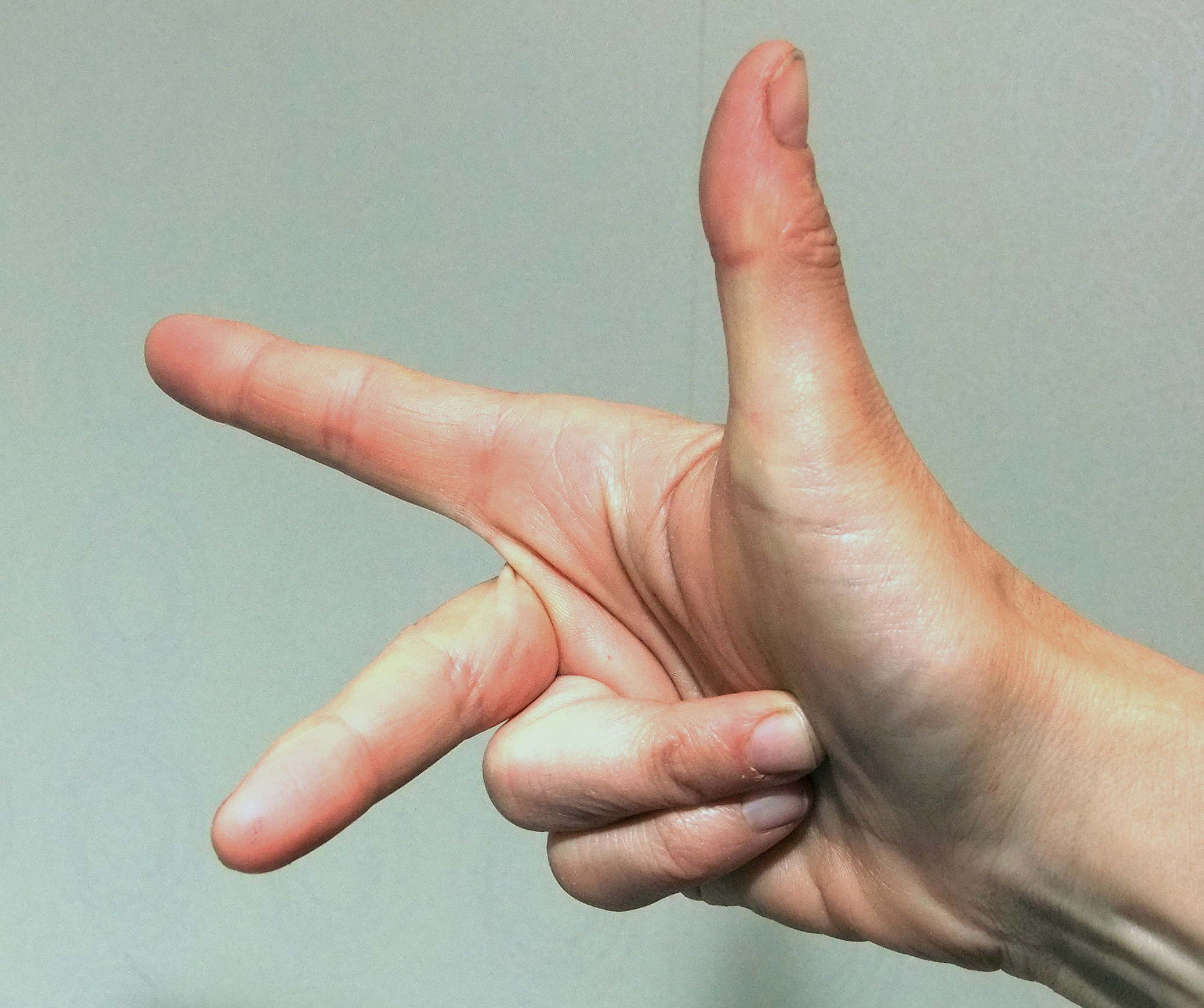
If ${\accentset{\rightharpoonup}{\boldsymbol{A}}}$ and ${\accentset{\rightharpoonup}{\boldsymbol{B}}}$ are perpendicular then $\theta_{AB}$ is $\pi/2$ , $\sin\theta_{AB}=1$ , and the magnitude of the cross product is $A B$ . If ${\accentset{\rightharpoonup}{\boldsymbol{A}}}$ and ${\accentset{\rightharpoonup}{\boldsymbol{B}}}$ are parallel then $\theta_{AB}$ is $0$ , $\sin\theta_{AB}=0$ and the cross product is ${\accentset{\rightharpoonup}{\boldsymbol{0}}}$ (the zero vector). This is why we say the cross product is a measure of the degree of orthogonality of two vectors.

Using the definition above you should be able to verify to your own satisfaction that ${\accentset{\rightharpoonup}{\boldsymbol{A}}}\times{\accentset{\rightharpoonup% }{\boldsymbol{B}}}=-{\accentset{\rightharpoonup}{\boldsymbol{B}}}\times{% \accentset{\rightharpoonup}{\boldsymbol{A}}}$ . Applying the definition to the standard base unit vectors you can see that $\hat{\boldsymbol{\imath}}\times\hat{\boldsymbol{\jmath}}=\hat{\boldsymbol{k}}$ , $\hat{\boldsymbol{\jmath}}\times\hat{\boldsymbol{k}}=\hat{\boldsymbol{\imath}}$ , and $\hat{\boldsymbol{k}}\times\hat{\boldsymbol{\imath}}=\hat{\boldsymbol{\jmath}}$ (fig. 1.71).

The geometric definition above and the geometric (tip to tail) definition of vector addition imply that the cross product follows the distributive rule, as explained in box 1.3 on page 1.3.

{\accentset{\rightharpoonup}{\boldsymbol{A}}}\times\left({\accentset{% \rightharpoonup}{\boldsymbol{B}}}+{\accentset{\rightharpoonup}{\boldsymbol{C}}% }\right)={\accentset{\rightharpoonup}{\boldsymbol{A}}}\times{\accentset{% \rightharpoonup}{\boldsymbol{B}}}+{\accentset{\rightharpoonup}{\boldsymbol{A}}% }\times{\accentset{\rightharpoonup}{\boldsymbol{C}}}.

Applying the distributive rule to the cross products of ${\accentset{\rightharpoonup}{\boldsymbol{A}}}=A_{x}\hat{\boldsymbol{\imath}}+A% _{y}\hat{\boldsymbol{\jmath}}+A_{z}\hat{\boldsymbol{k}}$ and ${\accentset{\rightharpoonup}{\boldsymbol{B}}}=B_{x}\hat{\boldsymbol{\imath}}+B% _{y}\hat{\boldsymbol{\jmath}}+B_{z}\hat{\boldsymbol{k}}$ leads to the algebraic formula for the Cartesian components of the cross product.

$\displaystyle{\accentset{\rightharpoonup}{\boldsymbol{A}}}\times{\accentset{% \rightharpoonup}{\boldsymbol{B}}}$	$\displaystyle=$	$\displaystyle\quad\![A_{y}B_{z}-A_{z}B_{y}]\hat{\boldsymbol{\imath}}$	(1.27)
		$\displaystyle+[A_{z}B_{x}-A_{x}B_{z}]\hat{\boldsymbol{\jmath}}$
		$\displaystyle+[A_{x}B_{y}-A_{y}B_{x}]\hat{\boldsymbol{k}}$

How the distributive rule is used to derive the component formula for cross product is also described in box 1.3 on page 1.3.

Memory aids for the component formula for cross product. There are various mnemonics for remembering the component formula for cross products. The most common is to calculate a ‘determinant’ of the $3\times 3$ matrix with one row given by $\hat{\boldsymbol{\imath}},\hat{\boldsymbol{\jmath}},\hat{\boldsymbol{k}}$ and the other two rows the components of ${\accentset{\rightharpoonup}{\boldsymbol{A}}}$ and ${\accentset{\rightharpoonup}{\boldsymbol{B}}}$ .

{\accentset{\rightharpoonup}{\boldsymbol{A}}}\times{\accentset{\rightharpoonup% }{\boldsymbol{B}}}=\det\left|\begin{array}[]{ccc}\hat{\boldsymbol{\imath}}&% \hat{\boldsymbol{\jmath}}&\hat{\boldsymbol{k}}\\ A_{x}&A_{y}&A_{z}\\ B_{x}&B_{y}&B_{z}\\ \end{array}\right|

Some key facts about cross products. The following identities and special cases of cross products are worth knowing well:

•

$(a{\accentset{\rightharpoonup}{\boldsymbol{A}}})\times{\accentset{% \rightharpoonup}{\boldsymbol{B}}}={\accentset{\rightharpoonup}{\boldsymbol{A}}% }\times(a{\accentset{\rightharpoonup}{\boldsymbol{B}}})=a({\accentset{% \rightharpoonup}{\boldsymbol{A}}}\times{\accentset{\rightharpoonup}{% \boldsymbol{B}}})$ (a distributive law)
•

${\accentset{\rightharpoonup}{\boldsymbol{A}}}\times{\accentset{\rightharpoonup% }{\boldsymbol{B}}}=-{\accentset{\rightharpoonup}{\boldsymbol{B}}}\times{% \accentset{\rightharpoonup}{\boldsymbol{A}}}$ (the cross product is not commutative!)
•

${\accentset{\rightharpoonup}{\boldsymbol{A}}}\times{\accentset{\rightharpoonup% }{\boldsymbol{B}}}={\accentset{\rightharpoonup}{\boldsymbol{0}}}\quad\hbox{if}% \quad{\accentset{\rightharpoonup}{\boldsymbol{A}}}\parallel{\accentset{% \rightharpoonup}{\boldsymbol{B}}}$ (parallel vectors have zero cross product)
•

$|{\accentset{\rightharpoonup}{\boldsymbol{A}}}\times{\accentset{% \rightharpoonup}{\boldsymbol{B}}}|=AB\quad\hbox{if}\quad{\accentset{% \rightharpoonup}{\boldsymbol{A}}}\perp{\accentset{\rightharpoonup}{\boldsymbol% {B}}}$
•

$\hat{\boldsymbol{\imath}}\times\hat{\boldsymbol{\jmath}}=\hat{\boldsymbol{k}},% \quad\hat{\boldsymbol{\jmath}}\times\hat{\boldsymbol{k}}=\hat{\boldsymbol{% \imath}},\quad\hat{\boldsymbol{k}}\times\hat{\boldsymbol{\imath}}=\hat{% \boldsymbol{\jmath}}$ (assuming the $x, y, z$ coordinate system is right handed — if you use your right hand and point your fingers along the positive $x$ axis, then curl them towards the positive $y$ axis, your thumb will point in the same direction as the positive $z$ axis. )
•

$\hat{\boldsymbol{\imath}}^{\prime}\times\hat{\boldsymbol{\jmath}}^{\prime}=% \hat{\boldsymbol{k}}^{\prime},\quad\hat{\boldsymbol{\jmath}}^{\prime}\times% \hat{\boldsymbol{k}}^{\prime}=\hat{\boldsymbol{\imath}}^{\prime},\quad\hat{% \boldsymbol{k}}^{\prime}\times\hat{\boldsymbol{\imath}}^{\prime}=\hat{% \boldsymbol{\jmath}}^{\prime}$
(assuming the $x^{\prime}y^{\prime}z^{\prime}$ coordinate system is right handed.)
•

$\hat{\boldsymbol{\imath}}\times\hat{\boldsymbol{\imath}}=\hat{\boldsymbol{% \jmath}}\times\hat{\boldsymbol{\jmath}}=\hat{\boldsymbol{k}}\times\hat{% \boldsymbol{k}}={\accentset{\rightharpoonup}{\boldsymbol{0}}}$ , $\hat{\boldsymbol{\imath}}^{\prime}\times\hat{\boldsymbol{\imath}}^{\prime}=% \hat{\boldsymbol{\jmath}}^{\prime}\times\hat{\boldsymbol{\jmath}}^{\prime}=% \hat{\boldsymbol{k}}^{\prime}\times\hat{\boldsymbol{k}}^{\prime}={\accentset{% \rightharpoonup}{\boldsymbol{0}}}$

The mixed triple product

The ‘mixed triple product’ of ${\accentset{\rightharpoonup}{\boldsymbol{A}}}$ , ${\accentset{\rightharpoonup}{\boldsymbol{B}}}$ , and ${\accentset{\rightharpoonup}{\boldsymbol{C}}}$ is so called because it mixes both the dot product and cross product in a single expression. The mixed triple product is also sometimes called the scalar triple product because its value is a scalar. The mixed triple product of ${\accentset{\rightharpoonup}{\boldsymbol{A}}}$ , ${\accentset{\rightharpoonup}{\boldsymbol{B}}}$ , and ${\accentset{\rightharpoonup}{\boldsymbol{C}}}$ is defined by and written as

{\accentset{\rightharpoonup}{\boldsymbol{A}}}\cdot\left({\accentset{% \rightharpoonup}{\boldsymbol{B}}}\times{\accentset{\rightharpoonup}{% \boldsymbol{C}}}\right)

and pronounced ‘A dot B cross C.’ The parentheses $()$ are sometimes omitted, i.e.,

{\accentset{\rightharpoonup}{\boldsymbol{A}}}\cdot{\accentset{\rightharpoonup}% {\boldsymbol{B}}}\times{\accentset{\rightharpoonup}{\boldsymbol{C}}},

because the wrong grouping $({\accentset{\rightharpoonup}{\boldsymbol{A}}}\cdot{\accentset{\rightharpoonup% }{\boldsymbol{B}}})\times{\accentset{\rightharpoonup}{\boldsymbol{C}}}$ is nonsense (you can’t take the cross product of a scalar with a vector) . It is apparent that one way of calculating the mixed triple product is to calculate the cross product of ${\accentset{\rightharpoonup}{\boldsymbol{B}}}$ and ${\accentset{\rightharpoonup}{\boldsymbol{C}}}$ and then to take the dot product of that result with ${\accentset{\rightharpoonup}{\boldsymbol{A}}}$ . Some people use the notation $\left({\accentset{\rightharpoonup}{\boldsymbol{A}}},{\accentset{% \rightharpoonup}{\boldsymbol{B}}},{\accentset{\rightharpoonup}{\boldsymbol{C}}% }\right)$ for the mixed triple product but it will not occur again in this book.

Filename:f92h7p1

Figure 1.72: One interpretation of the mixed triple product of

{\accentset{\rightharpoonup}{\boldsymbol{A}}}\times{\accentset{\rightharpoonup% }{\boldsymbol{B}}}\cdot{\accentset{\rightharpoonup}{\boldsymbol{C}}}

is as the volume (a scalar) of a parallelepiped with

{\accentset{\rightharpoonup}{\boldsymbol{A}}}

{\accentset{\rightharpoonup}{\boldsymbol{B}}}

, and

{\accentset{\rightharpoonup}{\boldsymbol{C}}}

as the three edges emanating from one corner. This interpretation only works if

{\accentset{\rightharpoonup}{\boldsymbol{A}}}

{\accentset{\rightharpoonup}{\boldsymbol{B}}}

, and

{\accentset{\rightharpoonup}{\boldsymbol{C}}}

are taken in the appropriate order, otherwise

{\accentset{\rightharpoonup}{\boldsymbol{A}}}\times{\accentset{\rightharpoonup% }{\boldsymbol{B}}}\cdot{\accentset{\rightharpoonup}{\boldsymbol{C}}}

is minus the volume which is calculated.

The mixed triple product has the same value if one takes the cross product of ${\accentset{\rightharpoonup}{\boldsymbol{A}}}$ and ${\accentset{\rightharpoonup}{\boldsymbol{B}}}$ and then the dot product of the result with ${\accentset{\rightharpoonup}{\boldsymbol{C}}}$ . That is ${\accentset{\rightharpoonup}{\boldsymbol{A}}}\cdot({\accentset{\rightharpoonup% }{\boldsymbol{B}}}\times{\accentset{\rightharpoonup}{\boldsymbol{C}}})=({% \accentset{\rightharpoonup}{\boldsymbol{A}}}\times{\accentset{\rightharpoonup}% {\boldsymbol{B}}})\cdot{\accentset{\rightharpoonup}{\boldsymbol{C}}}$ . This identity can be verified using the geometric description below, or by looking at the (complicated) expression for the mixed triple product of three general vectors ${\accentset{\rightharpoonup}{\boldsymbol{A}}}$ , ${\accentset{\rightharpoonup}{\boldsymbol{B}}}$ , and ${\accentset{\rightharpoonup}{\boldsymbol{C}}}$ in terms of their components as calculated the two different ways. One thus obtains the string of results

{\accentset{\rightharpoonup}{\boldsymbol{A}}}\cdot{\accentset{\rightharpoonup}% {\boldsymbol{B}}}\times{\accentset{\rightharpoonup}{\boldsymbol{C}}}={% \accentset{\rightharpoonup}{\boldsymbol{A}}}\times{\accentset{\rightharpoonup}% {\boldsymbol{B}}}\cdot{\accentset{\rightharpoonup}{\boldsymbol{C}}}=-{% \accentset{\rightharpoonup}{\boldsymbol{B}}}\times{\accentset{\rightharpoonup}% {\boldsymbol{A}}}\cdot{\accentset{\rightharpoonup}{\boldsymbol{C}}}=-{% \accentset{\rightharpoonup}{\boldsymbol{B}}}\cdot{\accentset{\rightharpoonup}{% \boldsymbol{A}}}\times{\accentset{\rightharpoonup}{\boldsymbol{C}}}=\ldots

The minus signs in the above expressions follow from the cross product identity that ${\accentset{\rightharpoonup}{\boldsymbol{A}}}\times{\accentset{\rightharpoonup% }{\boldsymbol{B}}}=-{\accentset{\rightharpoonup}{\boldsymbol{B}}}\times{% \accentset{\rightharpoonup}{\boldsymbol{A}}}$ .

The mixed triple product has various geometric interpretations, one of them is that ${\accentset{\rightharpoonup}{\boldsymbol{A}}}\cdot{\accentset{\rightharpoonup}% {\boldsymbol{B}}}\times{\accentset{\rightharpoonup}{\boldsymbol{C}}}$ is (plus or minus) the volume of the parallelepiped, the crooked shoe box, edged by ${\accentset{\rightharpoonup}{\boldsymbol{A}}}$ , ${\accentset{\rightharpoonup}{\boldsymbol{B}}}$ and ${\accentset{\rightharpoonup}{\boldsymbol{C}}}$ as shown in fig. 1.72.

Another way of calculating the value of the mixed triple product is with the determinant of a matrix whose rows are the components of the vectors.

{\accentset{\rightharpoonup}{\boldsymbol{A}}}\cdot({\accentset{\rightharpoonup% }{\boldsymbol{B}}}\times{\accentset{\rightharpoonup}{\boldsymbol{C}}})=\begin{% array}[]{|ccc|}A_{x}&A_{y}&A_{z}\\ B_{x}&B_{y}&B_{z}\\ C_{x}&C_{y}&C_{z}\\ \end{array}=\begin{array}[]{r}A_{x}(B_{y}C_{Z}-B_{z}C_{y})\\ +A_{y}(B_{z}C_{x}-B_{x}C_{z})\\ +A_{z}(B_{x}C_{y}-B_{y}C_{x})\\ \end{array}

The mixed triple product of three vectors is zero if

^†^†margin: In the language of linear algebra, the mixed triple product of three vectors is zero if the vectors are linearly dependent.

•

any two of them are parallel, or
•

all three of the vectors have one common plane.

Uses of the mixed triple product. The mixed triple product (or scalar triple product) is useful for calculating the moment of a force about an axis and for related dynamics quantities.

Vector triple product

A different triple product, sometimes called the ‘vector triple product’, ${\accentset{\rightharpoonup}{\boldsymbol{A}}}\times({\accentset{% \rightharpoonup}{\boldsymbol{B}}}\times{\accentset{\rightharpoonup}{% \boldsymbol{C}}})$ , is discussed later (in the Dynamics book).

Cross products and computers

The components of the cross product can be calculated with computer code that may look something like this.

    A = [  1  2  5 ]
    B = [ -2  4 19 ]
    C = [ ( A(2)*B(3) - A(3)*B(2) ) ...
          ( A(3)*B(1) - A(1)*B(3) ) ...
          ( A(1)*B(2) - A(2)*B(1) ) ]

giving the result C=[18 -29 8]. Many computer languages have a shorter way to write the cross product like cross(A,B). The mixed triple product might be calculated by assembling a $3\times 3$ matrix of rows and then taking a determinant like this:

        A   = [  1  2  5 ]
        B   = [ -2  4 19 ]
        C   = [ 32  4  5 ]
     matrix = [A ;     % Each row under the one above
               B ;
               C   ]
  mixedprod = det(matrix)

giving the result mixedprod = 500. A versatile computer language might allow a command like dot( A, cross(B,C) ) to calculate the mixed triple product.

Box 1.6 The cross product of vectors as matrix multiplication

For hand calculations in statics, this box is probably not useful. This box is for the theoretically inclined, and for people interested in doing complex dynamics calculations on a computer. We assume here that you know some linear algebra.

The cross product between two vectors ${\accentset{\rightharpoonup}{\boldsymbol{a}}}$ and ${\accentset{\rightharpoonup}{\boldsymbol{b}}}$ gives a new vector

{\accentset{\rightharpoonup}{\boldsymbol{c}}}={\accentset{\rightharpoonup}{% \boldsymbol{a}}}\times{\accentset{\rightharpoonup}{\boldsymbol{b}}}

All three of these vectors have components:

[{\accentset{\rightharpoonup}{\boldsymbol{a}}}]_{xy}=\left[\begin{array}[]{c}a% _{x}\\ a_{y}\\ a_{z}\end{array}\right],\quad[{\accentset{\rightharpoonup}{\boldsymbol{b}}}]_{% xy}=\left[\begin{array}[]{c}b_{x}\\ b_{y}\\ b_{z}\end{array}\right]

and

[{\accentset{\rightharpoonup}{\boldsymbol{c}}}]_{xy}=\left[\begin{array}[]{c}c% _{x}\\ c_{y}\\ c_{z}\end{array}\right].

The components of ${\accentset{\rightharpoonup}{\boldsymbol{c}}}$ can be calculated from those of ${\accentset{\rightharpoonup}{\boldsymbol{a}}}$ and ${\accentset{\rightharpoonup}{\boldsymbol{b}}}$ using the component rules from this section as

\left[\begin{array}[]{c}c_{x}\\ c_{y}\\ c_{z}\end{array}\right]\par=\par\left[\begin{array}[]{c}a_{y}b_{z}-a_{z}b_{y}% \\ a_{z}b_{x}-a_{x}b_{z}\\ a_{x}b_{y}-a_{y}b_{x}\end{array}\right].\par

Because the cross product ${\accentset{\rightharpoonup}{\boldsymbol{a}}}\times{\accentset{\rightharpoonup% }{\boldsymbol{b}}}$ is linear in ${\accentset{\rightharpoonup}{\boldsymbol{b}}}$ (meaning ${\accentset{\rightharpoonup}{\boldsymbol{a}}}\times({\accentset{% \rightharpoonup}{\boldsymbol{b}}}_{1}+{\accentset{\rightharpoonup}{\boldsymbol% {b}}}_{2})={\accentset{\rightharpoonup}{\boldsymbol{a}}}\times{\accentset{% \rightharpoonup}{\boldsymbol{b}}}_{1}+{\accentset{\rightharpoonup}{\boldsymbol% {a}}}\times{\accentset{\rightharpoonup}{\boldsymbol{b}}}_{2}$ , etc.) we can represent the cross product as some matrix times ${\accentset{\rightharpoonup}{\boldsymbol{b}}}$ .

We now define a matrix $[A]$ , that does the job. We associate the the vector ${\accentset{\rightharpoonup}{\boldsymbol{a}}}$ with the matrix $[A]$ as follows:

[A]\equiv\par\left[\begin{array}[]{ccc}0&-a_{z}&\phantom{-}a_{y}\\ \phantom{-}a_{z}&0&-a_{x}\\ -a_{y}&\phantom{-}a_{x}&0\end{array}\right].\par\par

(1.29)

$[A]$ is an anti-symmetric matrix (also called a skew symmetric matrix), with

[A]^{\prime}=-[A]\qquad\mbox{(A transpose is minus A)}.

The terms of $[A]$ on the diagonal are zero and those off the diagonal are negative of their corresponding (transposed) terms. The conversion rule (Equation 1.29) that takes a vector and puts its components in a matrix in the right place we can call $[\cal S]$ thus

[A]=[{\cal S}({\accentset{\rightharpoonup}{\boldsymbol{a}}})].

$[A]$ is the anti-symmetric matrix defined in terms of the components of ${\accentset{\rightharpoonup}{\boldsymbol{a}}}$ by $[{\cal S}({\accentset{\rightharpoonup}{\boldsymbol{a}}})]$ .

Just multiplying out the terms we see that

	$\displaystyle{\cal S}({\accentset{\rightharpoonup}{\boldsymbol{a}}})\times{% \accentset{\rightharpoonup}{\boldsymbol{b}}}$	$\displaystyle=\underbrace{\left[\begin{array}[]{ccc}0&-a_{z}&\phantom{-}a_{y}% \\ \phantom{-}a_{z}&0&-a_{x}\\ -a_{y}&\phantom{-}a_{x}&0\end{array}\right]}_{[{\cal S}({\accentset{% \rightharpoonup}{\boldsymbol{a}}})]}\par\left[\begin{array}[]{c}b_{x}\\ b_{y}\\ b_{z}\end{array}\right]$		(1.36)
		$\displaystyle=\par\left[\begin{array}[]{c}a_{y}b_{z}-a_{z}b_{y}\\ a_{z}b_{x}-a_{x}b_{z}\\ a_{x}b_{y}-a_{y}b_{x}\end{array}\right]\par.\par$		(1.40)

So we get our main result:

\par[{\accentset{\rightharpoonup}{\boldsymbol{a}}}\times{\accentset{% \rightharpoonup}{\boldsymbol{b}}}]_{xyz}=[{\cal S}({\accentset{\rightharpoonup% }{\boldsymbol{a}}})][{\accentset{\rightharpoonup}{\boldsymbol{b}}}]_{xyz}=[A][% {\accentset{\rightharpoonup}{\boldsymbol{b}}}]_{xyz}.\par

That is, the components of the cross product of ${\accentset{\rightharpoonup}{\boldsymbol{a}}}$ and ${\accentset{\rightharpoonup}{\boldsymbol{b}}}$ can be found by multiplying the matrix $[A]$ by the components of ${\accentset{\rightharpoonup}{\boldsymbol{b}}}$ .

Writing the cross product as a matrix multiplication is sometimes useful for dynamics when the first vector ${\accentset{\rightharpoonup}{\boldsymbol{a}}}$ is ${\accentset{\rightharpoonup}{\boldsymbol{\omega}}}$ (see box 16.2 on page 16.2). The advantage of the matrix representation over the cross product is that matrix multiplication satisfies the associative rule

[A]([B][C])=([A][B])[C]

whereas the vector cross product does not:

{\accentset{\rightharpoonup}{\boldsymbol{a}}}\times({\accentset{% \rightharpoonup}{\boldsymbol{b}}}\times{\accentset{\rightharpoonup}{% \boldsymbol{c}}})\neq({\accentset{\rightharpoonup}{\boldsymbol{a}}}\times{% \accentset{\rightharpoonup}{\boldsymbol{b}}})\times{\accentset{\rightharpoonup% }{\boldsymbol{c}}}.

Computer calculation

One could write a short program (computer function) that does the conversion from vector ${\accentset{\rightharpoonup}{\boldsymbol{a}}}$ to matrix $[A]={\cal S}({\accentset{\rightharpoonup}{\boldsymbol{a}}})$ and call it skew. That is, skew would calculate eqn. (1.29). Using skew we could carry out a cross product like this (see box 3.3 on page 3.3)

a = [1 2 3]’
b = [4 5 6]’
A = skew(a)
c = A*b Define vector ${\accentset{\rightharpoonup}{\boldsymbol{a}}}$ with components
Define vector ${\accentset{\rightharpoonup}{\boldsymbol{b}}}$ with components
Use the function skew’ to find A
Calculate the cross product ${\accentset{\rightharpoonup}{\boldsymbol{c}}}={\accentset{\rightharpoonup}{% \boldsymbol{a}}}\times{\accentset{\rightharpoonup}{\boldsymbol{b}}}$ using ordinary matrix multiplication.

For just one cross product this would be silly. But for a long calculation involving various vectors and matrices it often makes things simpler.

Box 1.7 The cross product: from geometry to components

Why is the 3D vector given by the component formula for the cross product ((1.27) on page 1.27)

[{\accentset{\rightharpoonup}{\boldsymbol{A}}}\times{\accentset{% \rightharpoonup}{\boldsymbol{B}}}]_{xyz}=\left[\begin{array}[]{c}(A_{y}B_{z}-A% _{z}B_{y})\\ (A_{z}B_{x}-A_{x}B_{z})\\ (A_{x}B_{y}-A_{y}B_{x})\end{array}\right]

(1.41)

the same vector as that given by the geometric definition ((1.24) on page 1.24),

{\accentset{\rightharpoonup}{\boldsymbol{A}}}\times{\accentset{\rightharpoonup% }{\boldsymbol{V}}}\equiv|{\accentset{\rightharpoonup}{\boldsymbol{A}}}||{% \accentset{\rightharpoonup}{\boldsymbol{V}}}|\sin{\theta_{AV}}\hat{\boldsymbol% {n}}_{\perp AV}?

Filename:tfigure1-cross2a

That these different-looking formulas should give the same answer is not obvious. Here we show why. Although the result is often used, the reasoning is not. But for logical completeness, and to entertain the curious, we present it here. We assume we know the geometric definition and want to find the component formula (1.41).

The reasoning has two big steps:

•

First we will show that the geometric definitions of the vector cross product ‘distributes’ over vector addition.
•

Then we apply the distributive rule to get our component formula.

A new definition of cross product

Start with ${\accentset{\rightharpoonup}{\boldsymbol{A}}}$ and ${\accentset{\rightharpoonup}{\boldsymbol{V}}}$ :

Filename:tfigure1-cross2e

Now we will show that the geometric formula

{\accentset{\rightharpoonup}{\boldsymbol{A}}}\times{\accentset{\rightharpoonup% }{\boldsymbol{V}}}\equiv|{\accentset{\rightharpoonup}{\boldsymbol{A}}}||{% \accentset{\rightharpoonup}{\boldsymbol{V}}}|\sin{\theta_{AV}}\hat{\boldsymbol% {n}}_{\perp AV}

is equivalent to a sequence of three operations: Project, rotate and stretch.

1.

Project ${\accentset{\rightharpoonup}{\boldsymbol{V}}}$ on to the plane P (normal to ${\accentset{\rightharpoonup}{\boldsymbol{A}}}$ ). The projection of ${\accentset{\rightharpoonup}{\boldsymbol{V}}}$ onto the plane orthogonal to ${\accentset{\rightharpoonup}{\boldsymbol{A}}}$ is ${\accentset{\rightharpoonup}{\boldsymbol{V}}}^{\prime}$ .

Filename:tfigure1-cross2d

The magnitude of ${\accentset{\rightharpoonup}{\boldsymbol{V}}}^{\prime}$ is

$|{\accentset{\rightharpoonup}{\boldsymbol{V}}}^{\prime}|=|{\accentset{% \rightharpoonup}{\boldsymbol{V}}}|\sin\theta_{AV}.$

${\accentset{\rightharpoonup}{\boldsymbol{V}}}^{\prime}$ is in the plane defined by ${\accentset{\rightharpoonup}{\boldsymbol{A}}}$ and ${\accentset{\rightharpoonup}{\boldsymbol{V}}}$ and also in the plane orthogonal to ${\accentset{\rightharpoonup}{\boldsymbol{A}}}$ .
2.

Then rotate that projection by $90^{{}^{\circ}}$ about ${\accentset{\rightharpoonup}{\boldsymbol{A}}}$ .

Filename:tfigure1-cross2c

Call the result of this rotation ${\accentset{\rightharpoonup}{\boldsymbol{V}}}^{\prime\prime}$ . The magnitude is unchanged by rotation so we still have

$|{\accentset{\rightharpoonup}{\boldsymbol{V}}}^{\prime\prime}|=|{\accentset{% \rightharpoonup}{\boldsymbol{V}}}|\sin\theta_{AV}.$

Note that ${\accentset{\rightharpoonup}{\boldsymbol{V}}}^{\prime\prime}$ is in the $\hat{\boldsymbol{n}}$ direction that is perpendicular to both ${\accentset{\rightharpoonup}{\boldsymbol{A}}}$ (it’s in the plane $\perp$ to ${\accentset{\rightharpoonup}{\boldsymbol{A}}}$ ) and to ${\accentset{\rightharpoonup}{\boldsymbol{V}}}$ (it’s rotated $90^{\circ}$ from ${\accentset{\rightharpoonup}{\boldsymbol{V}}}^{\prime}$ . So ${\accentset{\rightharpoonup}{\boldsymbol{V}}}^{\prime\prime}$ is in the direction of ${\accentset{\rightharpoonup}{\boldsymbol{A}}}\times{\accentset{\rightharpoonup% }{\boldsymbol{V}}}$ .
3.

Finally, stretch ${\accentset{\rightharpoonup}{\boldsymbol{V}}}^{\prime\prime}$ by $|{\accentset{\rightharpoonup}{\boldsymbol{A}}}|$ .

Filename:tfigure1-cross2b

This result has magnitude $|{\accentset{\rightharpoonup}{\boldsymbol{A}}}||{\accentset{\rightharpoonup}{% \boldsymbol{V}}}|\sin\theta_{AV}$ which is the magnitude of ${\accentset{\rightharpoonup}{\boldsymbol{A}}}\times{\accentset{\rightharpoonup% }{\boldsymbol{V}}}$ . This vector is in the direction normal to both ${\accentset{\rightharpoonup}{\boldsymbol{A}}}$ and ${\accentset{\rightharpoonup}{\boldsymbol{V}}}$ given by the right-hand rule, that’s the direction of ${\accentset{\rightharpoonup}{\boldsymbol{A}}}\times{\accentset{\rightharpoonup% }{\boldsymbol{V}}}$ . Having the same magnitude and direction as ${\accentset{\rightharpoonup}{\boldsymbol{A}}}\times{\accentset{\rightharpoonup% }{\boldsymbol{V}}}$ , it is ${\accentset{\rightharpoonup}{\boldsymbol{A}}}\times{\accentset{\rightharpoonup% }{\boldsymbol{V}}}$ . As infamously reasoned by Joseph McCarthy, “If it looks like a duck, walks like a duck and quacks like a duck,it’s a duck.”

Apply the new definition to ${\accentset{\rightharpoonup}{\boldsymbol{B}}}+{\accentset{\rightharpoonup}{% \boldsymbol{C}}}$

Consider ${\accentset{\rightharpoonup}{\boldsymbol{D}}}={\accentset{\rightharpoonup}{% \boldsymbol{B}}}+{\accentset{\rightharpoonup}{\boldsymbol{C}}}$ . We are interested in all three cross products: ${\accentset{\rightharpoonup}{\boldsymbol{A}}}\times{\accentset{\rightharpoonup% }{\boldsymbol{D}}}$ , ${\accentset{\rightharpoonup}{\boldsymbol{A}}}\times{\accentset{\rightharpoonup% }{\boldsymbol{B}}}$ , and ${\accentset{\rightharpoonup}{\boldsymbol{A}}}\times{\accentset{\rightharpoonup% }{\boldsymbol{C}}}$ .

Filename:tfigure1-crossc

First we will check that each of the operations above (project, rotate, stretch) is distributive.

1.

Project. The projection of a sum is the sum of the projections ( ${\accentset{\rightharpoonup}{\boldsymbol{D}}}^{\prime}={\accentset{% \rightharpoonup}{\boldsymbol{B}}}^{\prime}+{\accentset{\rightharpoonup}{% \boldsymbol{C}}}^{\prime}$ );

Filename:tfigure1-crossb
2.

Rotate. The sum of two $90^{{}^{\circ}}$ rotated vectors is the rotation of the sum ( ${\accentset{\rightharpoonup}{\boldsymbol{D}}}^{\prime\prime}={\accentset{% \rightharpoonup}{\boldsymbol{B}}}^{\prime\prime}+{\accentset{\rightharpoonup}{% \boldsymbol{C}}}^{\prime\prime}$ );

Filename:tfigure1-crossa
3.

Stretch. (stretched ${\accentset{\rightharpoonup}{\boldsymbol{D}}}^{\prime\prime}$ ) = (stretched ${\accentset{\rightharpoonup}{\boldsymbol{B}}}^{\prime\prime}$ ) + (stretched ${\accentset{\rightharpoonup}{\boldsymbol{C}}}^{\prime\prime}$ ), scalar multiplication is distributive.

Filename:tfigure1-cross

Thus the act of taking the cross product of ${\accentset{\rightharpoonup}{\boldsymbol{A}}}$ with ${\accentset{\rightharpoonup}{\boldsymbol{B}}}$ and adding that to the cross product of ${\accentset{\rightharpoonup}{\boldsymbol{A}}}$ with ${\accentset{\rightharpoonup}{\boldsymbol{C}}}$ gives the same result as taking the cross product of ${\accentset{\rightharpoonup}{\boldsymbol{A}}}$ with ${\accentset{\rightharpoonup}{\boldsymbol{D}}}\equiv{\accentset{\rightharpoonup% }{\boldsymbol{B}}}+{\accentset{\rightharpoonup}{\boldsymbol{C}}}$ . That’s the distributive law for vector cross products over vector addition:

{\accentset{\rightharpoonup}{\boldsymbol{A}}}\quad\times\quad\left({\accentset% {\rightharpoonup}{\boldsymbol{B}}}+{\accentset{\rightharpoonup}{\boldsymbol{C}% }}\right)\quad=\quad{\accentset{\rightharpoonup}{\boldsymbol{A}}}\times{% \accentset{\rightharpoonup}{\boldsymbol{B}}}\quad+\quad{\accentset{% \rightharpoonup}{\boldsymbol{A}}}\times{\accentset{\rightharpoonup}{% \boldsymbol{C}}}.

The distributive rule also works for a sum of 3 or more vectors (all of the reasoning above would be the same). And that the distributive rule works when the sum is on the left (i.e., that $({\accentset{\rightharpoonup}{\boldsymbol{B}}}+{\accentset{\rightharpoonup}{% \boldsymbol{C}}})\times{\accentset{\rightharpoonup}{\boldsymbol{A}}}={% \accentset{\rightharpoonup}{\boldsymbol{B}}}\times{\accentset{\rightharpoonup}% {\boldsymbol{A}}}+{\accentset{\rightharpoonup}{\boldsymbol{C}}}\times{% \accentset{\rightharpoonup}{\boldsymbol{A}}})$ also follows by very similar reasoning, so we skip those details. In sum, we know now that $({\accentset{\rightharpoonup}{\boldsymbol{A}}}+{\accentset{\rightharpoonup}{% \boldsymbol{B}}}+{\accentset{\rightharpoonup}{\boldsymbol{C}}})\times({% \accentset{\rightharpoonup}{\boldsymbol{D}}}+{\accentset{\rightharpoonup}{% \boldsymbol{E}}}+{\accentset{\rightharpoonup}{\boldsymbol{F}}})={\accentset{% \rightharpoonup}{\boldsymbol{A}}}\times{\accentset{\rightharpoonup}{% \boldsymbol{D}}}+{\accentset{\rightharpoonup}{\boldsymbol{A}}}\times{% \accentset{\rightharpoonup}{\boldsymbol{E}}}+\dots$ (9 terms in all).

Applying the distributive rule to the vectors’ components

A vector is a sum of component parts. First note that

{\accentset{\rightharpoonup}{\boldsymbol{A}}}=A_{x}\hat{\boldsymbol{\imath}}+A% _{y}\hat{\boldsymbol{\jmath}}+A_{z}\hat{\boldsymbol{k}}\qquad\mbox{and}\qquad{% \accentset{\rightharpoonup}{\boldsymbol{B}}}=B_{x}\hat{\boldsymbol{\imath}}+B_% {y}\hat{\boldsymbol{\jmath}}+B_{z}\hat{\boldsymbol{k}}

From the distributive rule (demonstrated with the 8 pictures above) we know that

{\accentset{\rightharpoonup}{\boldsymbol{A}}}\times{\accentset{\rightharpoonup% }{\boldsymbol{B}}}=[A_{x}\hat{\boldsymbol{\imath}}+A_{y}\hat{\boldsymbol{% \jmath}}+A_{z}\hat{\boldsymbol{k}}]\times[B_{x}\hat{\boldsymbol{\imath}}+B_{y}% \hat{\boldsymbol{\jmath}}+B_{z}\hat{\boldsymbol{k}}].

Now we just apply the distributive law, using what we know about the cross products of $\hat{\boldsymbol{\imath}},\hat{\boldsymbol{\jmath}}$ and $\hat{\boldsymbol{k}}$ with each other (e.g., that $\hat{\boldsymbol{\imath}}\times\hat{\boldsymbol{\imath}}={\accentset{% \rightharpoonup}{\boldsymbol{0}}}$ and that $\hat{\boldsymbol{\imath}}\times\hat{\boldsymbol{\jmath}}=\hat{\boldsymbol{k}}$ ).

First in 2D, to better show the patterns in the algebra:

$\displaystyle{\accentset{\rightharpoonup}{\boldsymbol{A}}}\times{\accentset{% \rightharpoonup}{\boldsymbol{B}}}$	$\displaystyle=$	$\displaystyle[A_{x}\hat{\boldsymbol{\imath}}+A_{y}\hat{\boldsymbol{\jmath}}]% \times[B_{x}\hat{\boldsymbol{\imath}}+B_{y}\hat{\boldsymbol{\jmath}}]$
	$\displaystyle=$	$\displaystyle[A_{x}\hat{\boldsymbol{\imath}}+A_{y}\hat{\boldsymbol{\jmath}}]% \times B_{x}\hat{\boldsymbol{\imath}}+[A_{x}\hat{\boldsymbol{\imath}}+A_{y}% \hat{\boldsymbol{\jmath}}]\times B_{y}\hat{\boldsymbol{\jmath}}$
	$\displaystyle=$	$\displaystyle\quad\!A_{x}B_{x}\hat{\boldsymbol{\imath}}\times\hat{\boldsymbol{% \imath}}+A_{x}B_{y}\hat{\boldsymbol{\imath}}\times\hat{\boldsymbol{\jmath}}$
		$\displaystyle+A_{y}B_{x}\hat{\boldsymbol{\jmath}}\times\hat{\boldsymbol{\imath% }}+A_{y}B_{y}\hat{\boldsymbol{\jmath}}\times\hat{\boldsymbol{\jmath}}$
	$\displaystyle=$	$\displaystyle\quad\!A_{x}B_{x}{\accentset{\rightharpoonup}{\boldsymbol{0}}}+A_% {x}B_{y}\hat{\boldsymbol{k}}-A_{y}B_{x}\hat{\boldsymbol{k}}+A_{y}B_{y}{% \accentset{\rightharpoonup}{\boldsymbol{0}}}$

So ${\accentset{\rightharpoonup}{\boldsymbol{A}}}\times{\accentset{\rightharpoonup% }{\boldsymbol{B}}}=[A_{x}B_{y}-A_{y}B_{x}]\hat{\boldsymbol{k}}$ (2D)

Now in 3D, applying the distributive rule multiple times,

$\displaystyle{\accentset{\rightharpoonup}{\boldsymbol{A}}}\times{\accentset{% \rightharpoonup}{\boldsymbol{B}}}$	$\displaystyle=$	$\displaystyle[A_{x}\hat{\boldsymbol{\imath}}+A_{y}\hat{\boldsymbol{\jmath}}+A_% {z}\hat{\boldsymbol{k}}]\times[B_{x}\hat{\boldsymbol{\imath}}+B_{y}\hat{% \boldsymbol{\jmath}}+B_{z}\hat{\boldsymbol{k}}]$
	$\displaystyle=$	$\displaystyle\quad\!A_{x}B_{x}\hat{\boldsymbol{\imath}}\times\hat{\boldsymbol{% \imath}}+A_{x}B_{y}\hat{\boldsymbol{\imath}}\times\hat{\boldsymbol{\jmath}}+A_% {x}B_{z}\hat{\boldsymbol{\imath}}\times\hat{\boldsymbol{k}}$
		$\displaystyle+A_{y}B_{x}\hat{\boldsymbol{\jmath}}\times\hat{\boldsymbol{\imath% }}+A_{y}B_{y}\hat{\boldsymbol{\jmath}}\times\hat{\boldsymbol{\jmath}}+A_{y}B_{% z}\hat{\boldsymbol{\jmath}}\times\hat{\boldsymbol{k}}$
		$\displaystyle+A_{z}B_{x}\hat{\boldsymbol{k}}\times\hat{\boldsymbol{\imath}}+A_% {z}B_{y}\hat{\boldsymbol{k}}\times\hat{\boldsymbol{\jmath}}+A_{z}B_{z}\hat{% \boldsymbol{k}}\times\hat{\boldsymbol{k}}$
	$\displaystyle=$	$\displaystyle\quad\!A_{x}B_{x}{\accentset{\rightharpoonup}{\boldsymbol{0}}}+A_% {x}B_{y}\hat{\boldsymbol{k}}-A_{x}B_{z}\hat{\boldsymbol{\jmath}}$
		$\displaystyle-A_{y}B_{x}\hat{\boldsymbol{k}}+A_{y}B_{y}{\accentset{% \rightharpoonup}{\boldsymbol{0}}}+A_{y}B_{z}\hat{\boldsymbol{\imath}}$
		$\displaystyle+A_{z}B_{x}\hat{\boldsymbol{\jmath}}-A_{z}B_{y}\hat{\boldsymbol{% \imath}}+A_{z}B_{z}{\accentset{\rightharpoonup}{\boldsymbol{0}}}\par$

$\displaystyle\mbox{So\qquad}{\accentset{\rightharpoonup}{\boldsymbol{A}}}% \times{\accentset{\rightharpoonup}{\boldsymbol{B}}}=\phantom{+}$	$\displaystyle[A_{y}B_{z}-A_{z}B_{y}]\hat{\boldsymbol{\imath}}$	(1.42)
$\displaystyle+$	$\displaystyle[A_{z}B_{x}-A_{x}B_{z}]\hat{\boldsymbol{\jmath}}$	(1.43)
$\displaystyle+$	$\displaystyle[A_{x}B_{y}-A_{y}B_{x}]\hat{\boldsymbol{k}}$	(1.44)

from which you can pick out the familiar $x y z$ components of the cross product. As hoped, we have derived the component formula for the cross product from its geometric definition.

[The other way around. On the other hand, if we are given the component formula we can (almost) verify that it corresponds to the geometric definition: Use the component formulas for the magnitude, dot product and cross product (1.1,1.2& 1.41) and tediously evaluate $|{\accentset{\rightharpoonup}{\boldsymbol{A}}}\times{\accentset{% \rightharpoonup}{\boldsymbol{B}}}|^{2}$ and note that it is equal to $|{\accentset{\rightharpoonup}{\boldsymbol{A}}}|^{2}|{\accentset{% \rightharpoonup}{\boldsymbol{B}}}|^{2}-|{\accentset{\rightharpoonup}{% \boldsymbol{A}}}\cdot{\accentset{\rightharpoonup}{\boldsymbol{B}}}|^{2}.$ . Because we already know that $|{\accentset{\rightharpoonup}{\boldsymbol{A}}}\cdot{\accentset{\rightharpoonup% }{\boldsymbol{B}}}|=|{\accentset{\rightharpoonup}{\boldsymbol{A}}}||{% \accentset{\rightharpoonup}{\boldsymbol{B}}}|\cos\theta$ and that $\sin^{2}\theta=1-\cos^{2}\theta$ this gives $|{\accentset{\rightharpoonup}{\boldsymbol{A}}}\times{\accentset{% \rightharpoonup}{\boldsymbol{B}}}|=|{\accentset{\rightharpoonup}{\boldsymbol{A% }}}||{\accentset{\rightharpoonup}{\boldsymbol{B}}}||\sin\theta|$ . To show that ${\accentset{\rightharpoonup}{\boldsymbol{A}}}\times{\accentset{\rightharpoonup% }{\boldsymbol{B}}}$ is orthogonal to ${\accentset{\rightharpoonup}{\boldsymbol{A}}}$ and ${\accentset{\rightharpoonup}{\boldsymbol{B}}}$ use the component formulas to show that $({\accentset{\rightharpoonup}{\boldsymbol{A}}}\times{\accentset{% \rightharpoonup}{\boldsymbol{B}}})\cdot{\accentset{\rightharpoonup}{% \boldsymbol{A}}}=0$ and $({\accentset{\rightharpoonup}{\boldsymbol{A}}}\times{\accentset{% \rightharpoonup}{\boldsymbol{B}}})\cdot{\accentset{\rightharpoonup}{% \boldsymbol{B}}}=0$ . A final tricky point, which we skip here, is that the component formula obeys the right hand, as opposed to the left hand, rule.]

SAMPLE 1.17 Cross product in 2-D: Two vectors ⇀ a and ⇀ b of length 10 $\,\mathrm{ft}$ and 6 $\,\mathrm{ft}$ , respectively, are shown in the figure. The angle between the two vectors is $\theta=60^{\circ}$ . Find the cross product ${\accentset{\rightharpoonup}{\boldsymbol{a}}}\times{\accentset{\rightharpoonup% }{\boldsymbol{b}}}$ .

Filename:pfigure-blue-52-2

Figure 1.73:

Solution Both vectors ⇀ a and ⇀ b are in the $x y$ plane. Therefore, their cross product will point in either $+\hat{\boldsymbol{k}}$ or $-\hat{\boldsymbol{k}}$ direction (normal to the plane formed by ${\accentset{\rightharpoonup}{\boldsymbol{a}}}$ and ${\accentset{\rightharpoonup}{\boldsymbol{b}}}$ ). To determine the direction of the normal, we use the right hand rule and curl our fingers from ${\accentset{\rightharpoonup}{\boldsymbol{a}}}$ towards ${\accentset{\rightharpoonup}{\boldsymbol{b}}}$ , tracing angle $\theta$ counterclockwise. The thumb then points in the positive $\hat{\boldsymbol{k}}$ direction, indicating $\hat{\boldsymbol{n}}=\hat{\boldsymbol{k}}$ . Thus,

$\displaystyle{\accentset{\rightharpoonup}{\boldsymbol{a}}}\times{\accentset{% \rightharpoonup}{\boldsymbol{b}}}$	$\displaystyle=$	$\displaystyle\|{\accentset{\rightharpoonup}{\boldsymbol{a}}}\|\|{\accentset{% \rightharpoonup}{\boldsymbol{b}}}\|\sin\theta\hat{\boldsymbol{n}}$
	$\displaystyle=$	$\displaystyle(10\,\mathrm{ft})\cdot(6\,\mathrm{ft})\cdot\sin 60^{\circ}\hat{% \boldsymbol{k}}$
	$\displaystyle=$	$\displaystyle 60\,\mathrm{ft}^{2}\cdot\frac{\sqrt{3}}{2}\hat{\boldsymbol{k}}$
	$\displaystyle=$	$\displaystyle 30\sqrt{3}\,\mathrm{ft}^{2}\hat{\boldsymbol{k}}.$

Answer: ${\accentset{\rightharpoonup}{\boldsymbol{a}}}\times{\accentset{\rightharpoonup% }{\boldsymbol{b}}}=30\sqrt{3}\,\mathrm{ft}^{2}\hat{\boldsymbol{k}}$

SAMPLE 1.18

Filename:pfigure4-4-rp16

Figure 1.74:

Computing 2-D cross product in different ways: The two vectors shown in the figure are ${\accentset{\rightharpoonup}{\boldsymbol{a}}}=2\hat{\boldsymbol{\imath}}-\hat{% \boldsymbol{\jmath}}$ and ${\accentset{\rightharpoonup}{\boldsymbol{b}}}=4\hat{\boldsymbol{\imath}}+2\hat% {\boldsymbol{\jmath}}$ . The angle between the two vectors turns out to be $\theta=\sin^{-1}(4/5)$ . Find the cross product ${\accentset{\rightharpoonup}{\boldsymbol{a}}}\times{\accentset{\rightharpoonup% }{\boldsymbol{b}}}$

1.

using the angle $\theta$ , and
2.

using the components of the vectors.

Solution

Cross product using the angle $\theta$ :

$\displaystyle{\accentset{\rightharpoonup}{\boldsymbol{a}}}\times{\accentset{% \rightharpoonup}{\boldsymbol{b}}}$	$\displaystyle=$	$\displaystyle\|{\accentset{\rightharpoonup}{\boldsymbol{a}}}\|\|{\accentset{% \rightharpoonup}{\boldsymbol{b}}}\|\sin\theta\hat{\boldsymbol{n}}$
	$\displaystyle=$	$\displaystyle\|2\hat{\boldsymbol{\imath}}-\hat{\boldsymbol{\jmath}}\|\|4\hat{% \boldsymbol{\imath}}+2\hat{\boldsymbol{\jmath}}\|\cdot\sin(\sin^{-1}\frac{4}{5}% )\hat{\boldsymbol{k}}$
	$\displaystyle=$	$\displaystyle(\sqrt{2^{2}+1^{2}})(\sqrt{4^{2}+2^{2}})\cdot\frac{4}{5}\hat{% \boldsymbol{k}}$
	$\displaystyle=$	$\displaystyle\sqrt{5}\cdot\sqrt{20}\cdot\frac{4}{5}\hat{\boldsymbol{k}}=10% \cdot\frac{4}{5}\hat{\boldsymbol{k}}$
	$\displaystyle=$	$\displaystyle 8\hat{\boldsymbol{k}}.$

Cross product using components:

$\displaystyle{\accentset{\rightharpoonup}{\boldsymbol{a}}}\times{\accentset{% \rightharpoonup}{\boldsymbol{b}}}$	$\displaystyle=$	$\displaystyle(2\hat{\boldsymbol{\imath}}-\hat{\boldsymbol{\jmath}})\times(4% \hat{\boldsymbol{\imath}}+2\hat{\boldsymbol{\jmath}})$
	$\displaystyle=$	$\displaystyle 2\hat{\boldsymbol{\imath}}\times(4\hat{\boldsymbol{\imath}}+2% \hat{\boldsymbol{\jmath}})-\hat{\boldsymbol{\jmath}}\times(4\hat{\boldsymbol{% \imath}}+2\hat{\boldsymbol{\jmath}})$
	$\displaystyle=$	$\displaystyle 8\underbrace{\hat{\boldsymbol{\imath}}\times\hat{\boldsymbol{% \imath}}}_{{\accentset{\rightharpoonup}{\boldsymbol{0}}}}+4\underbrace{\hat{% \boldsymbol{\imath}}\times\hat{\boldsymbol{\jmath}}}_{\hat{\boldsymbol{k}}}-4% \underbrace{\hat{\boldsymbol{\jmath}}\times\hat{\boldsymbol{\imath}}}_{-\hat{% \boldsymbol{k}}}-2\underbrace{\hat{\boldsymbol{\jmath}}\times\hat{\boldsymbol{% \jmath}}}_{{\accentset{\rightharpoonup}{\boldsymbol{0}}}}$
	$\displaystyle=$	$\displaystyle 4\hat{\boldsymbol{k}}+4\hat{\boldsymbol{k}}$
	$\displaystyle=$	$\displaystyle 8\hat{\boldsymbol{k}}.$

The answers obtained from the two methods are, of course, the same as they must be.

Answer: ${\accentset{\rightharpoonup}{\boldsymbol{a}}}\times{\accentset{\rightharpoonup% }{\boldsymbol{b}}}=8\hat{\boldsymbol{k}}$

SAMPLE 1.19 Find the shortest distance from a point to a line: A straight line passes through two points, A (-1,1) and B (2,2), in the $x y$ plane. Find the shortest distance from the origin to the line.

Filename:pfigure4-4-rp14

Figure 1.75:

Solution There are various ways we can find the required distance. In 2-D, the following two methods can be used for quick calculations.

Method-1:

Filename:pfigure4-4-rp15

Figure 1.76:

The shortest distance $d$ between a point P and a given line AB is obtained by taking the dot product of a vector from P to any point on the line with a unit normal to the given line. Thus, $d=\hat{\boldsymbol{n}}\cdot{\accentset{\rightharpoonup}{\boldsymbol{r}}}_{\!% \mathrm{A}}=\hat{\boldsymbol{n}}\cdot{\accentset{\rightharpoonup}{\boldsymbol{% r}}}_{\!\mathrm{B}}$ where $\hat{\boldsymbol{n}}$ is a unit vector normal to ${\accentset{\rightharpoonup}{\boldsymbol{r}}}_{\!\mathrm{B/A}}$ . Why?

From geometry we know that the shortest distance from a given point to a given line is the perpendicular distance from the line to the given point. Thus to find this distance, we need to draw a perpendicular from the given point to the line of interest. In fig. 1.76, this distance $d$ is shown as line OC. From the figure, we also see that $d=$ OC $=$ OB $\cos\alpha$ , that is, $d$ is the projection of vector ${\accentset{\rightharpoonup}{\boldsymbol{r}}}_{\!\mathrm{B}}$ along OC. But OC is normal to AB, hence, we can find a unit vector $\hat{\boldsymbol{n}}$ along OC by finding a normal to vector ${\accentset{\rightharpoonup}{\boldsymbol{r}}}_{\!\mathrm{B/A}}$ . Thus,

d={\accentset{\rightharpoonup}{\boldsymbol{r}}}_{\!\mathrm{B}}\cdot\hat{% \boldsymbol{n}},\quad\mbox{where}\quad\hat{\boldsymbol{n}}\perp{\accentset{% \rightharpoonup}{\boldsymbol{r}}}_{\!\mathrm{B/A}}.

We can use cross product to find $\hat{\boldsymbol{n}}$ . Since ${\accentset{\rightharpoonup}{\boldsymbol{r}}}_{\!\mathrm{B/A}}$ is in the $x y$ plane, $\hat{\boldsymbol{k}}\times{\accentset{\rightharpoonup}{\boldsymbol{r}}}_{\!% \mathrm{B/A}}$ gives us a vector perpendicular to AB and in the $x y$ plane. Thus,

\hat{\boldsymbol{n}}=\frac{\hat{\boldsymbol{k}}\times{\accentset{% \rightharpoonup}{\boldsymbol{r}}}_{\!\mathrm{B/A}}}{|\hat{\boldsymbol{k}}% \times{\accentset{\rightharpoonup}{\boldsymbol{r}}}_{\!\mathrm{B/A}}|},\par% \quad\mbox{and hence,}\quad\par d={\accentset{\rightharpoonup}{\boldsymbol{r}}% }_{\!\mathrm{B}}\cdot\frac{\hat{\boldsymbol{k}}\times{\accentset{% \rightharpoonup}{\boldsymbol{r}}}_{\!\mathrm{B/A}}}{|\hat{\boldsymbol{k}}% \times{\accentset{\rightharpoonup}{\boldsymbol{r}}}_{\!\mathrm{B/A}}|}.

From the given coordinates, ${\accentset{\rightharpoonup}{\boldsymbol{r}}}_{\!\mathrm{B}}=2\hat{\boldsymbol% {\imath}}+2\hat{\boldsymbol{\jmath}}$ and ${\accentset{\rightharpoonup}{\boldsymbol{r}}}_{\!\mathrm{B/A}}={\accentset{% \rightharpoonup}{\boldsymbol{r}}}_{\!\mathrm{B}}-{\accentset{\rightharpoonup}{% \boldsymbol{r}}}_{\!\mathrm{A}}=3\hat{\boldsymbol{\imath}}+\hat{\boldsymbol{% \jmath}}$ , we get

	$\displaystyle\hat{\boldsymbol{n}}$	$\displaystyle=$	$\displaystyle\frac{\hat{\boldsymbol{k}}\times(3\hat{\boldsymbol{\imath}}+\hat{% \boldsymbol{\jmath}})}{\|\hat{\boldsymbol{k}}\times(3\hat{\boldsymbol{\imath}}+% \hat{\boldsymbol{\jmath}})\|}=\frac{3\hat{\boldsymbol{\jmath}}-\hat{\boldsymbol% {\imath}}}{\|3\hat{\boldsymbol{\jmath}}-\hat{\boldsymbol{\imath}}\|}=-\frac{1}{% \sqrt{10}}\hat{\boldsymbol{\imath}}+\frac{3}{\sqrt{10}}\hat{\boldsymbol{\jmath}}$
	$\displaystyle d$	$\displaystyle=$	$\displaystyle{\accentset{\rightharpoonup}{\boldsymbol{r}}}_{\!\mathrm{B}}\cdot% \hat{\boldsymbol{n}}=(2\hat{\boldsymbol{\imath}}+2\hat{\boldsymbol{\jmath}})% \cdot\left(-\frac{1}{\sqrt{10}}\hat{\boldsymbol{\imath}}+\frac{3}{\sqrt{10}}% \hat{\boldsymbol{\jmath}}\right)=\frac{4}{\sqrt{10}}.$

Answer: $d=\frac{4}{\sqrt{10}}$

You can easily verify that we get the same result even if we use ${\accentset{\rightharpoonup}{\boldsymbol{r}}}_{\!\mathrm{A}}$ in place of ${\accentset{\rightharpoonup}{\boldsymbol{r}}}_{\!\mathrm{B}}$ (or for that matter, any vector from O to a point on line AB). For example, ${\accentset{\rightharpoonup}{\boldsymbol{r}}}_{\!\mathrm{A}}\cdot\hat{% \boldsymbol{n}}=(-ui+\hat{\boldsymbol{\jmath}})\cdot(-\hat{\boldsymbol{\imath}% }+3\hat{\boldsymbol{\jmath}})/\sqrt{10}=4/\sqrt{10}$ , the same value as obtained above.

Method-2:

Filename:tfigure4-spherical-rotaxis

Figure 1.77:

The shortest distance between a point P and a given line AB can also be found by taking a cross product of a unit vector $\hat{\boldsymbol{\lambda}}_{\mathrm{AB}}$ along the line with any vector from P to a point on the line, e.g., ${\accentset{\rightharpoonup}{\boldsymbol{r}}}_{\!\mathrm{B/P}}$ . For the given case, where P is the origin, we get, $d=\hat{\boldsymbol{\lambda}}_{\mathrm{AB}}\times{\accentset{\rightharpoonup}{% \boldsymbol{r}}}_{\!\mathrm{B}}$ . Why?

From fig. 1.77, we see that $d\equiv{\rm OC=OB}\sin\theta$ where $\theta$ is the angle between ${\accentset{\rightharpoonup}{\boldsymbol{r}}}_{\!\mathrm{B}}$ and ${\accentset{\rightharpoonup}{\boldsymbol{r}}}_{\!\mathrm{B/A}}$ . Let $\hat{\boldsymbol{\lambda}}_{\mathrm{AB}}$ be a unit vector along line AB. Then,

\hat{\boldsymbol{\lambda}}_{\mathrm{AB}}\times{\accentset{\rightharpoonup}{% \boldsymbol{r}}}_{\!\mathrm{B}}=\underbrace{|\hat{\boldsymbol{\lambda}}_{% \mathrm{AB}}|}_{1}|{\accentset{\rightharpoonup}{\boldsymbol{r}}}_{\!\mathrm{B}% }|\sin\theta\hat{\boldsymbol{n}}=|{\accentset{\rightharpoonup}{\boldsymbol{r}}% }_{\!\mathrm{B}}|\sin\theta\hat{\boldsymbol{k}}.

Thus, $d=OB\sin\theta=|{\accentset{\rightharpoonup}{\boldsymbol{r}}}_{\!\mathrm{B}}|% \sin\theta=|\hat{\boldsymbol{\lambda}}_{\mathrm{AB}}\times{\accentset{% \rightharpoonup}{\boldsymbol{r}}}_{\!\mathrm{B}}|$ . We can, therefore, compute $d$ easily by computing the cross product as follows.

	$\displaystyle d$	$\displaystyle=$	$\displaystyle\|\hat{\boldsymbol{\lambda}}_{\mathrm{AB}}\times{\accentset{% \rightharpoonup}{\boldsymbol{r}}}_{\!\mathrm{B}}\|=\left\|(\frac{3\hat{% \boldsymbol{\imath}}+\hat{\boldsymbol{\jmath}}}{\sqrt{3^{2}+1^{2}}})\times(2% \hat{\boldsymbol{\imath}}+2\hat{\boldsymbol{\jmath}})\right\|$
		$\displaystyle=$	$\displaystyle\left\|\frac{4}{\sqrt{10}}\hat{\boldsymbol{k}}\right\|=\frac{4}{% \sqrt{10}}.$

which is the same answer as obtained by Method-1. Once again, you can verify that $\hat{\boldsymbol{\lambda}}_{\mathrm{AB}}\times{\accentset{\rightharpoonup}{% \boldsymbol{r}}}_{\!\mathrm{A}}$ also gives the same answer.

Answer: $d=4/\sqrt{10}$

SAMPLE 1.20 Computing cross product in 3-D: Compute ${\accentset{\rightharpoonup}{\boldsymbol{a}}}\times{\accentset{\rightharpoonup% }{\boldsymbol{b}}}$ , where ${\accentset{\rightharpoonup}{\boldsymbol{a}}}=\hat{\boldsymbol{\imath}}+\hat{% \boldsymbol{\jmath}}-2\hat{\boldsymbol{k}}$ and ${\accentset{\rightharpoonup}{\boldsymbol{b}}}=3\hat{\boldsymbol{\imath}}+-4% \hat{\boldsymbol{\jmath}}+\hat{\boldsymbol{k}}$ .

Solution The calculation of a cross product between two 3-D vectors can be carried out by either using a determinant or the distributive rule. Usually, if the vectors involved have just one or two components, it is easier to use the distributive rule. We show you both methods here and encourage you to learn both. We are given two vectors:

	$\displaystyle{\accentset{\rightharpoonup}{\boldsymbol{a}}}$	$\displaystyle=$	$\displaystyle a_{1}\hat{\boldsymbol{\imath}}+a_{2}\hat{\boldsymbol{\jmath}}+a_% {3}\hat{\boldsymbol{k}}=\hat{\boldsymbol{\imath}}+\hat{\boldsymbol{\jmath}}-2% \hat{\boldsymbol{k}},$
	$\displaystyle{\accentset{\rightharpoonup}{\boldsymbol{b}}}$	$\displaystyle=$	$\displaystyle b_{1}\hat{\boldsymbol{\imath}}+b_{2}\hat{\boldsymbol{\jmath}}+b_% {3}\hat{\boldsymbol{k}}=3\hat{\boldsymbol{\imath}}+-4\hat{\boldsymbol{\jmath}}% +\hat{\boldsymbol{k}}.$

•

Calculation using the determinant formula: In this method, we first write a $3\times 3$ matrix whose first row has the basis vectors as its elements, the second row has the components of the first vector as its elements, and the third row has the components of the second vector as its elements. Thus,

$\displaystyle{{\accentset{\rightharpoonup}{\boldsymbol{a}}}\times{\accentset{% \rightharpoonup}{\boldsymbol{b}}}}$	$\displaystyle=$	$\displaystyle\left\|\begin{array}[]{ccc}\hat{\boldsymbol{\imath}}&\hat{% \boldsymbol{\jmath}}&\hat{\boldsymbol{k}}\\ a_{1}&a_{2}&a_{3}\\ b_{1}&b_{2}&b_{3}\end{array}\right\|$
	$\displaystyle=$	$\displaystyle\hat{\boldsymbol{\imath}}(a_{2}b_{3}-a_{3}b_{2})+\hat{\boldsymbol% {\jmath}}(a_{3}b_{1}-a_{1}b_{3})+\hat{\boldsymbol{k}}(a_{1}b_{2}-b_{1}a_{2})$
	$\displaystyle=$	$\displaystyle\hat{\boldsymbol{\imath}}(1-8)+\hat{\boldsymbol{\jmath}}(-6-1)+% \hat{\boldsymbol{k}}(-4-3)$
	$\displaystyle=$	$\displaystyle-7(\hat{\boldsymbol{\imath}}+\hat{\boldsymbol{\jmath}}+\hat{% \boldsymbol{k}}).$

•

Calculation using the distributive rule: In this method, we carry out the cross product by distributing the cross product properly over the three basis vectors. The steps involved are shown below.

Filename:tfigure5-7

Figure 1.78: The cross product of any two basis vectors is positive in the direction of the arrow and negative if carried out backwards, e.g.

\hat{\boldsymbol{\imath}}\times\hat{\boldsymbol{\jmath}}=\hat{\boldsymbol{k}}

but

\hat{\boldsymbol{\jmath}}\times\hat{\boldsymbol{\imath}}=-\hat{\boldsymbol{k}}

$\displaystyle{{\accentset{\rightharpoonup}{\boldsymbol{a}}}\times{\accentset{% \rightharpoonup}{\boldsymbol{b}}}}$	$\displaystyle=$	$\displaystyle(a_{1}\hat{\boldsymbol{\imath}}+a_{2}\hat{\boldsymbol{\jmath}}+a_% {3}\hat{\boldsymbol{k}})\times(b_{1}\hat{\boldsymbol{\imath}}+b_{2}\hat{% \boldsymbol{\jmath}}+b_{3}\hat{\boldsymbol{k}})$
	$\displaystyle=$	$\displaystyle a_{1}\hat{\boldsymbol{\imath}}\times(b_{1}\hat{\boldsymbol{% \imath}}+b_{2}\hat{\boldsymbol{\jmath}}+b_{3}\hat{\boldsymbol{k}})+$
		$\displaystyle a_{2}\hat{\boldsymbol{\jmath}}\times(b_{1}\hat{\boldsymbol{% \imath}}+b_{2}\hat{\boldsymbol{\jmath}}+b_{3}\hat{\boldsymbol{k}})+$
		$\displaystyle a_{3}\hat{\boldsymbol{k}}\times(b_{1}\hat{\boldsymbol{\imath}}+b% _{2}\hat{\boldsymbol{\jmath}}+b_{3}\hat{\boldsymbol{k}})$
	$\displaystyle=$	$\displaystyle a_{1}b_{1}(\overbrace{\hat{\boldsymbol{\imath}}\times\hat{% \boldsymbol{\imath}}}^{\bf 0})+a_{1}b_{2}(\overbrace{\hat{\boldsymbol{\imath}}% \times\hat{\boldsymbol{\jmath}}}^{\hat{\boldsymbol{k}}})+a_{1}b_{3}(\overbrace% {\hat{\boldsymbol{\imath}}\times\hat{\boldsymbol{k}}}^{-\hat{\boldsymbol{% \jmath}}})+$
		$\displaystyle a_{2}b_{1}(\overbrace{\hat{\boldsymbol{\jmath}}\times\hat{% \boldsymbol{\imath}}}^{-\hat{\boldsymbol{k}}})+a_{2}b_{2}(\overbrace{\hat{% \boldsymbol{\jmath}}\times\hat{\boldsymbol{\jmath}}}^{\bf 0})+a_{2}b_{3}(% \overbrace{\hat{\boldsymbol{\jmath}}\times\hat{\boldsymbol{k}}}^{\hat{% \boldsymbol{\imath}}})+$
		$\displaystyle a_{3}b_{1}(\overbrace{\hat{\boldsymbol{k}}\times\hat{\boldsymbol% {\imath}}}^{\hat{\boldsymbol{\jmath}}})+a_{3}b_{2}(\overbrace{\hat{\boldsymbol% {k}}\times\hat{\boldsymbol{\jmath}}}^{-\hat{\boldsymbol{\imath}}})+a_{3}b_{3}(% \overbrace{\hat{\boldsymbol{k}}\times\hat{\boldsymbol{k}}}^{\bf 0})$
	$\displaystyle=$	$\displaystyle\hat{\boldsymbol{\imath}}(a_{2}b_{3}-a_{3}b_{2})+\hat{\boldsymbol% {\jmath}}(a_{3}b_{1}-a_{1}b_{3})+\hat{\boldsymbol{k}}(a_{1}b_{2}-b_{1}a_{2})$
	$\displaystyle=$	$\displaystyle\hat{\boldsymbol{\imath}}(1-8)+\hat{\boldsymbol{\jmath}}(-6-1)+% \hat{\boldsymbol{k}}(-4-3)$
	$\displaystyle=$	$\displaystyle-7(\hat{\boldsymbol{\imath}}+\hat{\boldsymbol{\jmath}}+\hat{% \boldsymbol{k}})$

which, of course, is the same result as obtained above using the determinant. Making a sketch such as Fig. 1.78 is helpful while calculating cross products this way. The product of any two basis vectors is positive in the direction of the arrow and negative if carried out backwards, e.g., $\hat{\boldsymbol{\imath}}\times\hat{\boldsymbol{\jmath}}=\hat{\boldsymbol{k}}$ but $\hat{\boldsymbol{\jmath}}\times\hat{\boldsymbol{\imath}}=-\hat{\boldsymbol{k}}$ .

Answer: ${{\accentset{\rightharpoonup}{\boldsymbol{a}}}\times{\accentset{% \rightharpoonup}{\boldsymbol{b}}}}=-7(\hat{\boldsymbol{\imath}}+\hat{% \boldsymbol{\jmath}}+\hat{\boldsymbol{k}})$

SAMPLE 1.21 Finding a vector normal to two given vectors: Find a unit vector perpendicular to the vectors ${\accentset{\rightharpoonup}{\boldsymbol{r}}}_{A}=\hat{\boldsymbol{\imath}}-2% \hat{\boldsymbol{\jmath}}+\hat{\boldsymbol{k}}$ and ${\accentset{\rightharpoonup}{\boldsymbol{r}}}_{b}=3\hat{\boldsymbol{\jmath}}+2% \hat{\boldsymbol{k}}$ .

Solution The cross product between two vectors gives a vector perpendicular to the plane formed by the two vectors. The sense of direction is determined by the right hand rule.

Let ${\accentset{\rightharpoonup}{\boldsymbol{N}}}=N\hat{\boldsymbol{\lambda}}$ be the perpendicular vector.

$\displaystyle{\accentset{\rightharpoonup}{\boldsymbol{N}}}$	$\displaystyle=$	$\displaystyle{\accentset{\rightharpoonup}{\boldsymbol{r}}}_{A}\times{% \accentset{\rightharpoonup}{\boldsymbol{r}}}_{B}$
	$\displaystyle=$	$\displaystyle(\hat{\boldsymbol{\imath}}-2\hat{\boldsymbol{\jmath}}+\hat{% \boldsymbol{k}})\times(3\hat{\boldsymbol{\jmath}}+2\hat{\boldsymbol{k}})$
	$\displaystyle=\text{ This calculation can be done in either of the two ways % shown in the previous sample.}$	$\displaystyle-7\hat{\boldsymbol{\imath}}-2\hat{\boldsymbol{\jmath}}+3\hat{% \boldsymbol{k}}.$

Therefore,

$\displaystyle\hat{\boldsymbol{\lambda}}$	$\displaystyle=$	$\displaystyle\frac{{\accentset{\rightharpoonup}{\boldsymbol{N}}}}{N}$
	$\displaystyle=$	$\displaystyle\frac{-7\hat{\boldsymbol{\imath}}-2\hat{\boldsymbol{\jmath}}+3% \hat{\boldsymbol{k}}}{\sqrt{7^{2}+2^{2}+3^{2}}}$
	$\displaystyle=$	$\displaystyle-0.89\hat{\boldsymbol{\imath}}-0.25\hat{\boldsymbol{\jmath}}+0.38% \hat{\boldsymbol{k}}$

Answer: $\hat{\boldsymbol{\lambda}}=-0.89\hat{\boldsymbol{\imath}}-0.25\hat{\boldsymbol% {\jmath}}+0.38\hat{\boldsymbol{k}}$

Check:

•

$|\hat{\boldsymbol{\lambda}}|=(0.89)^{2}+(0.25)^{2}+(0.38)^{2}\mathrel{\mathop{% =}\limits^{\surd}}1.$ (it is a unit vector)
•

$\hat{\boldsymbol{\lambda}}\cdot{\accentset{\rightharpoonup}{\boldsymbol{r}}}_{% A}=1(-0.89)-2(-0.25)+1(0.38)\mathrel{\mathop{=}\limits^{\surd}}0.$ $(\hat{\boldsymbol{\lambda}}\perp{\accentset{\rightharpoonup}{\boldsymbol{r}}}_% {A}).$
•

$\hat{\boldsymbol{\lambda}}\cdot{\accentset{\rightharpoonup}{\boldsymbol{r}}}_{% B}=3(-0.25)+2(0.38)\mathrel{\mathop{=}\limits^{\surd}}0.$ $(\hat{\boldsymbol{\lambda}}\perp{\accentset{\rightharpoonup}{\boldsymbol{r}}}_% {B}).$

Comments: If ˆ λ is perpendicular to ${\accentset{\rightharpoonup}{\boldsymbol{r}}}_{\!\mathrm{A}}$ and ${\accentset{\rightharpoonup}{\boldsymbol{r}}}_{\!\mathrm{B}}$ , then so is $-\hat{\boldsymbol{\lambda}}$ . The perpendicularity does not change by changing the sense of direction (from positive to negative) of the vector. In fact, if $\hat{\boldsymbol{\lambda}}$ is perpendicular to a vector ${\accentset{\rightharpoonup}{\boldsymbol{r}}}$ then any scalar multiple of ˆ λ , i.e., $\alpha\hat{\boldsymbol{\lambda}}$ , is also perpendicular to ${\accentset{\rightharpoonup}{\boldsymbol{r}}}$ . This follows because

\alpha\hat{\boldsymbol{\lambda}}\cdot{\accentset{\rightharpoonup}{\boldsymbol{% r}}}=\alpha(\hat{\boldsymbol{\lambda}}\cdot{\accentset{\rightharpoonup}{% \boldsymbol{r}}})=\alpha(0)=0.

The case of $-\hat{\boldsymbol{\lambda}}$ is just a particular instance of this rule with $\alpha=-1$ .

SAMPLE 1.22 Finding a vector normal to a plane: Find a unit vector normal to the plane ABC shown in the figure.

Filename:tfigure5-gen-rigid-body

Figure 1.79:

Solution A vector normal to the plane ABC would be normal to any vector in that plane. In particular, if we take any two vectors, say ${\accentset{\rightharpoonup}{\boldsymbol{r}}}_{\!\mathrm{AB}}$ and ${\accentset{\rightharpoonup}{\boldsymbol{r}}}_{\!\mathrm{AC}}$ , the normal to the plane would be perpendicular to both ${\accentset{\rightharpoonup}{\boldsymbol{r}}}_{\!\mathrm{AB}}$ and ${\accentset{\rightharpoonup}{\boldsymbol{r}}}_{\!\mathrm{AC}}$ . Since the cross product of two vectors gives a vector perpendicular to both vectors, we can find the desired normal vector by taking the cross product of ${\accentset{\rightharpoonup}{\boldsymbol{r}}}_{\!\mathrm{AB}}$ and ${\accentset{\rightharpoonup}{\boldsymbol{r}}}_{\!\mathrm{AC}}$ . Thus,

$\displaystyle{\accentset{\rightharpoonup}{\boldsymbol{N}}}$	$\displaystyle=$	$\displaystyle{\accentset{\rightharpoonup}{\boldsymbol{r}}}_{\!\mathrm{AB}}% \times{\accentset{\rightharpoonup}{\boldsymbol{r}}}_{\!\mathrm{AC}}$
	$\displaystyle=$	$\displaystyle(\hat{\boldsymbol{\imath}}-\hat{\boldsymbol{k}})\times(\hat{% \boldsymbol{\jmath}}-\hat{\boldsymbol{k}})$
	$\displaystyle=$	$\displaystyle\underbrace{\hat{\boldsymbol{\imath}}\times\hat{\boldsymbol{% \jmath}}}_{\hat{\boldsymbol{k}}}-\underbrace{\hat{\boldsymbol{\imath}}\times% \hat{\boldsymbol{k}}}_{-\hat{\boldsymbol{\jmath}}}-\underbrace{\hat{% \boldsymbol{k}}\times\hat{\boldsymbol{\jmath}}}_{-\hat{\boldsymbol{\imath}}}+% \underbrace{\hat{\boldsymbol{k}}\times\hat{\boldsymbol{k}}}_{{\accentset{% \rightharpoonup}{\boldsymbol{0}}}}$
	$\displaystyle=$	$\displaystyle\hat{\boldsymbol{\imath}}+\hat{\boldsymbol{\jmath}}+\hat{% \boldsymbol{k}}$
$\displaystyle\hbox to36.135pt{\hfil$\Rightarrow$\hfil}\hat{\boldsymbol{n}}$	$\displaystyle=$	$\displaystyle\frac{{\accentset{\rightharpoonup}{\boldsymbol{N}}}}{\|{\accentset% {\rightharpoonup}{\boldsymbol{N}}}\|}$
	$\displaystyle=$	$\displaystyle\frac{1}{\sqrt{3}}(\hat{\boldsymbol{\imath}}+\hat{\boldsymbol{% \jmath}}+\hat{\boldsymbol{k}}).$

Answer: $\hat{\boldsymbol{n}}=\frac{1}{\sqrt{3}}(\hat{\boldsymbol{\imath}}+\hat{% \boldsymbol{\jmath}}+\hat{\boldsymbol{k}})$

Check: Now let us check if ˆ n is normal to any vector in the plane ABC. It is fairly easy to show that $\hat{\boldsymbol{n}}\cdot{\accentset{\rightharpoonup}{\boldsymbol{r}}}_{\!% \mathrm{AB}}=\hat{\boldsymbol{n}}\cdot{\accentset{\rightharpoonup}{\boldsymbol% {r}}}_{\!\mathrm{AC}}=0$ . This is not a surprise because we found ˆ n from the cross product of ${\accentset{\rightharpoonup}{\boldsymbol{r}}}_{\!\mathrm{AB}}$ and ${\accentset{\rightharpoonup}{\boldsymbol{r}}}_{\!\mathrm{AC}}$ . Let us check if ˆ n is normal to ${\accentset{\rightharpoonup}{\boldsymbol{r}}}_{\!\mathrm{BC}}$ :

$\displaystyle\hat{\boldsymbol{n}}\cdot{\accentset{\rightharpoonup}{\boldsymbol% {r}}}_{\!\mathrm{BC}}$	$\displaystyle=$	$\displaystyle\frac{1}{\sqrt{3}}(\hat{\boldsymbol{\imath}}+\hat{\boldsymbol{% \jmath}}+\hat{\boldsymbol{k}})\cdot(-\hat{\boldsymbol{\imath}}+\hat{% \boldsymbol{\jmath}})$
	$\displaystyle=$	$\displaystyle\frac{1}{\sqrt{3}}(-\hat{\boldsymbol{\imath}}\cdot\hat{% \boldsymbol{\imath}}+\hat{\boldsymbol{\jmath}}\cdot\hat{\boldsymbol{\jmath}})$
	$\displaystyle=$	$\displaystyle\frac{1}{\sqrt{3}}(-1+1)\mathrel{\mathop{=}\limits^{\surd}}0.$

SAMPLE 1.23

Filename:tfigure5-term1-a

Figure 1.80:

The shortest distance between two lines: Two lines, AB and CD, in 3-D space are defined by four specified points, A(0,2 $\,\mathrm{m}$ ,1 $\,\mathrm{m}$ ), B(2 $\,\mathrm{m}$ ,1 $\,\mathrm{m}$ ,3 $\,\mathrm{m}$ ), C(-1 $\,\mathrm{m}$ ,0,0), and D(2 $\,\mathrm{m}$ ,2 $\,\mathrm{m}$ ,2 $\,\mathrm{m}$ ) as shown in the figure. Find the shortest distance between the two lines (which are the infinite extensions of the segments shown).

Solution The shortest distance between any pair of lines is the length of the line that is perpendicular to both the lines. We can find the shortest distance in three steps:

1.

First find a vector that is perpendicular to both the lines. This is easy. Take two vectors ${\accentset{\rightharpoonup}{\boldsymbol{r}}}_{\!\mathrm{1}}\qquad\mbox{and}% \qquad{\accentset{\rightharpoonup}{\boldsymbol{r}}}_{\!\mathrm{2}}$ , one along each of the two given lines. Take the cross product of the two vectors and normalize the result to get unit vector $\hat{\boldsymbol{n}}$ .
2.

Find a vector parallel to ˆ n that connects the two lines. This is a little tricky. We don’t know where to start on any of the two lines. However, we can take any vector from one line to the other and then, take its component along ˆ n .
3.

Find the length (magnitude) of the vector just found (in the direction of ˆ n ). This is simply the component we find in step (b) devoid of its sign.

Now let us carry out these steps on the given problem.

Step-1: Find a unit vector ˆ n that is perpendicular to both the lines.

$\displaystyle{\accentset{\rightharpoonup}{\boldsymbol{r}}}_{\!\mathrm{AB}}$	$\displaystyle=$	$\displaystyle 2\,\mathrm{m}\hat{\boldsymbol{\imath}}-1\,\mathrm{m}\hat{% \boldsymbol{\jmath}}+2\,\mathrm{m}\hat{\boldsymbol{k}}$
$\displaystyle{\accentset{\rightharpoonup}{\boldsymbol{r}}}_{\!\mathrm{CD}}$	$\displaystyle=$	$\displaystyle 3\,\mathrm{m}\hat{\boldsymbol{\imath}}+2\,\mathrm{m}\hat{% \boldsymbol{\jmath}}+2\,\mathrm{m}\hat{\boldsymbol{k}}$
$\displaystyle\hbox to36.135pt{\hfil$\Rightarrow$\hfil}{\accentset{% \rightharpoonup}{\boldsymbol{r}}}_{\!\mathrm{AB}}\times{\accentset{% \rightharpoonup}{\boldsymbol{r}}}_{\!\mathrm{CD}}$	$\displaystyle=$	$\displaystyle\begin{array}[t]{\|rrr\|}\hat{\boldsymbol{\imath}}&\hat{\boldsymbol% {\jmath}}&\hat{\boldsymbol{k}}\\ 2&-1&2\\ 3&2&2\end{array}\;\,\mathrm{m}^{2}$
	$\displaystyle=$	$\displaystyle\hat{\boldsymbol{\imath}}(-2-4)\,\mathrm{m}^{2}+\hat{\boldsymbol{% \jmath}}(6-4)\,\mathrm{m}^{2}+\hat{\boldsymbol{k}}(4+3)\,\mathrm{m}^{2}\hskip 5% 6.9055pt$
	$\displaystyle=$	$\displaystyle(-6\hat{\boldsymbol{\imath}}+2\hat{\boldsymbol{\jmath}}+7\hat{% \boldsymbol{k}})\,\mathrm{m}^{2}$

$\displaystyle\hat{\boldsymbol{n}}$	$\displaystyle=$	$\displaystyle\frac{{\accentset{\rightharpoonup}{\boldsymbol{r}}}_{\!\mathrm{AB% }}\times{\accentset{\rightharpoonup}{\boldsymbol{r}}}_{\!\mathrm{CD}}}{\|{% \accentset{\rightharpoonup}{\boldsymbol{r}}}_{\!\mathrm{AB}}\times{\accentset{% \rightharpoonup}{\boldsymbol{r}}}_{\!\mathrm{CD}}\|}$
	$\displaystyle=$	$\displaystyle\frac{1}{\sqrt{89}}(-6\hat{\boldsymbol{\imath}}+2\hat{\boldsymbol% {\jmath}}+7\hat{\boldsymbol{k}}).$

Step-2: Find any vector from one line to the other line and find its component along ˆ n .

$\displaystyle{\accentset{\rightharpoonup}{\boldsymbol{r}}}_{\!\mathrm{AC}}$	$\displaystyle=$	$\displaystyle-1\,\mathrm{m}\hat{\boldsymbol{\imath}}-2\,\mathrm{m}\hat{% \boldsymbol{\jmath}}-1\,\mathrm{m}\hat{\boldsymbol{k}}$
$\displaystyle{\accentset{\rightharpoonup}{\boldsymbol{r}}}_{\!\mathrm{AC}}% \cdot\hat{\boldsymbol{n}}$	$\displaystyle=$	$\displaystyle-(\hat{\boldsymbol{\imath}}+2\hat{\boldsymbol{\jmath}}+\hat{% \boldsymbol{k}})\,\mathrm{m}\cdot\frac{1}{\sqrt{89}}(-6\hat{\boldsymbol{\imath% }}+2\hat{\boldsymbol{\jmath}}+7\hat{\boldsymbol{k}})$
	$\displaystyle=$	$\displaystyle\frac{1}{\sqrt{89}}(6-4-7)\,\mathrm{m}=-\frac{5}{\sqrt{89}}\,% \mathrm{m}.$

3.

Step-3: Find the required distance $d$ by taking the magnitude of the component along ˆ n .

$d=\left|{\accentset{\rightharpoonup}{\boldsymbol{r}}}_{\!\mathrm{AC}}\cdot\hat% {\boldsymbol{n}}\right|=\left|-\frac{5}{\sqrt{89}}\,\mathrm{m}\right|=0.53\,% \mathrm{m}$

Answer: $d=0.53\,\mathrm{m}$

SAMPLE 1.24 The mixed triple product: Calculate the mixed triple product $\hat{\boldsymbol{\lambda}}\cdot({\accentset{\rightharpoonup}{\boldsymbol{a}}}% \times{\accentset{\rightharpoonup}{\boldsymbol{b}}})$ for $\hat{\boldsymbol{\lambda}}=\frac{1}{\sqrt{2}}(\hat{\boldsymbol{\imath}}+\hat{% \boldsymbol{\jmath}}),\;{\accentset{\rightharpoonup}{\boldsymbol{a}}}=3\hat{% \boldsymbol{\imath}}$ , and ${\accentset{\rightharpoonup}{\boldsymbol{b}}}=\hat{\boldsymbol{\imath}}+\hat{% \boldsymbol{\jmath}}+3\hat{\boldsymbol{k}}.$

Solution We compute the given mixed triple product in two ways here:

•

Method-1: Straight calculation using cross product and dot product.

$\displaystyle\mbox{Let}\qquad{\accentset{\rightharpoonup}{\boldsymbol{c}}}$	$\displaystyle=$	$\displaystyle{\accentset{\rightharpoonup}{\boldsymbol{a}}}\times{\accentset{% \rightharpoonup}{\boldsymbol{b}}}$
	$\displaystyle=$	$\displaystyle(3\hat{\boldsymbol{\imath}})\times(\hat{\boldsymbol{\imath}}+\hat% {\boldsymbol{\jmath}}+3\hat{\boldsymbol{k}})$
	$\displaystyle=$	$\displaystyle 3\underbrace{\hat{\boldsymbol{\imath}}\times\hat{\boldsymbol{% \imath}}}_{{\accentset{\rightharpoonup}{\boldsymbol{0}}}}+3\underbrace{\hat{% \boldsymbol{\imath}}\times\hat{\boldsymbol{\jmath}}}_{\hat{\boldsymbol{k}}}+9% \underbrace{\hat{\boldsymbol{\imath}}\times\hat{\boldsymbol{k}}}_{-\hat{% \boldsymbol{\jmath}}}$
	$\displaystyle=$	$\displaystyle-9\hat{\boldsymbol{\jmath}}+3\hat{\boldsymbol{k}}$
$\displaystyle\mbox{So,}\qquad\hat{\boldsymbol{\lambda}}\cdot({\accentset{% \rightharpoonup}{\boldsymbol{a}}}\times{\accentset{\rightharpoonup}{% \boldsymbol{b}}})$	$\displaystyle=$	$\displaystyle\hat{\boldsymbol{\lambda}}\cdot{\accentset{\rightharpoonup}{% \boldsymbol{c}}}$
	$\displaystyle=$	$\displaystyle\frac{1}{\sqrt{2}}(\hat{\boldsymbol{\imath}}+\hat{\boldsymbol{% \jmath}})\cdot(-9\hat{\boldsymbol{\jmath}}+3\hat{\boldsymbol{k}})$
	$\displaystyle=$	$\displaystyle\frac{1}{\sqrt{2}}(-9\underbrace{\hat{\boldsymbol{\imath}}\cdot% \hat{\boldsymbol{\jmath}}}_{0}+3\underbrace{\hat{\boldsymbol{\imath}}\cdot\hat% {\boldsymbol{k}}}_{0}-9\underbrace{\hat{\boldsymbol{\jmath}}\cdot\hat{% \boldsymbol{\jmath}}}_{1}+3\underbrace{\hat{\boldsymbol{\jmath}}\cdot\hat{% \boldsymbol{k}}}_{0})$
	$\displaystyle=$	$\displaystyle-\frac{9}{\sqrt{2}}.$

Answer: $\hat{\boldsymbol{\lambda}}\cdot({\accentset{\rightharpoonup}{\boldsymbol{a}}}% \times{\accentset{\rightharpoonup}{\boldsymbol{b}}})=-\frac{9}{\sqrt{2}}$

•

Method-2: Using the determinant formula for mixed product.

$\displaystyle\hat{\boldsymbol{\lambda}}\cdot({\accentset{\rightharpoonup}{% \boldsymbol{a}}}\times{\accentset{\rightharpoonup}{\boldsymbol{b}}})$ $\displaystyle=$ $\displaystyle\begin{array}[t]{|rrr|}\lambda_{x}&\lambda_{y}&\lambda_{z}\\ a_{x}&a_{y}&a_{z}\\ b_{x}&b_{y}&b_{z}\end{array}$

$\displaystyle=$ $\displaystyle\begin{array}[t]{|rrr|}\frac{1}{\sqrt{2}}&\frac{1}{\sqrt{2}}&0\\ 3&0&0\\ 1&1&3\end{array}$

$\displaystyle=$ $\displaystyle\frac{1}{\sqrt{2}}(0-0)+\frac{1}{\sqrt{2}}(0-9)+0$

$\displaystyle=$ $\displaystyle-\frac{9}{\sqrt{2}}.$

Answer: $\hat{\boldsymbol{\lambda}}\cdot({\accentset{\rightharpoonup}{\boldsymbol{a}}}% \times{\accentset{\rightharpoonup}{\boldsymbol{b}}})=-\frac{9}{\sqrt{2}}$

Problems for 1.3 Vector Cross Product

1.3.1 Find the cross product of the two vectors shown in the figures below from the information given in the figures.

Filename:tfigure5-term1-b

Figure 1.81

1.3.2 Vector algebra. For each equation below state whether:

1.

The equation is nonsense. If so, why?
2.

Is always true. Why? Give an example.
3.

Is never true. Why? Give an example.
4.

Is sometimes true. Give examples both ways.

You may use trivial examples.

(a)

${\accentset{\rightharpoonup}{\boldsymbol{B}}}\times{\accentset{\rightharpoonup% }{\boldsymbol{C}}}={\accentset{\rightharpoonup}{\boldsymbol{C}}}\times{% \accentset{\rightharpoonup}{\boldsymbol{B}}}$
(b)

${\accentset{\rightharpoonup}{\boldsymbol{B}}}\times{\accentset{\rightharpoonup% }{\boldsymbol{C}}}={\accentset{\rightharpoonup}{\boldsymbol{C}}}\cdot{% \accentset{\rightharpoonup}{\boldsymbol{B}}}$
(c)

${\accentset{\rightharpoonup}{\boldsymbol{C}}}\cdot({\accentset{\rightharpoonup% }{\boldsymbol{A}}}\times{\accentset{\rightharpoonup}{\boldsymbol{B}}})={% \accentset{\rightharpoonup}{\boldsymbol{B}}}\cdot({\accentset{\rightharpoonup}% {\boldsymbol{C}}}\times{\accentset{\rightharpoonup}{\boldsymbol{A}}})$
(d)

${\accentset{\rightharpoonup}{\boldsymbol{A}}}\times({\accentset{% \rightharpoonup}{\boldsymbol{B}}}\times{\accentset{\rightharpoonup}{% \boldsymbol{C}}})=({\accentset{\rightharpoonup}{\boldsymbol{A}}}\cdot{% \accentset{\rightharpoonup}{\boldsymbol{C}}}){\accentset{\rightharpoonup}{% \boldsymbol{B}}}-({\accentset{\rightharpoonup}{\boldsymbol{A}}}\cdot{% \accentset{\rightharpoonup}{\boldsymbol{B}}}){\accentset{\rightharpoonup}{% \boldsymbol{C}}}$

1.3.3 What do you get when you cross a vector and a scalar? Answer: No partial credit.

1.3.4 Carry out the following cross products in different ways and determine which method takes the least amount of time for you.

(a)

${\accentset{\rightharpoonup}{\boldsymbol{r}}}=2.0\,\mathrm{ft}\hat{\boldsymbol% {\imath}}+3.0\,\mathrm{ft}\hat{\boldsymbol{\jmath}}-1.5\,\mathrm{ft}\hat{% \boldsymbol{k}};\;{\accentset{\rightharpoonup}{\boldsymbol{F}}}=-0.3\,{\rm lbf% }\hat{\boldsymbol{\imath}}-1.0\,{\rm lbf}\hat{\boldsymbol{k}};\;\ {\accentset{% \rightharpoonup}{\boldsymbol{r}}}\times{\accentset{\rightharpoonup}{% \boldsymbol{F}}}=?$
(b)

${\accentset{\rightharpoonup}{\boldsymbol{r}}}=(-\hat{\boldsymbol{\imath}}+2.0% \hat{\boldsymbol{\jmath}}+0.4\hat{\boldsymbol{k}})\,\mathrm{m};\;{\accentset{% \rightharpoonup}{\boldsymbol{L}}}=(3.5\hat{\boldsymbol{\jmath}}-2.0\hat{% \boldsymbol{k}})\,\mathrm{kg}\,\mathrm{m}/\mathrm{s};\ {\accentset{% \rightharpoonup}{\boldsymbol{r}}}\times{\accentset{\rightharpoonup}{% \boldsymbol{L}}}=?$
(c)

${\accentset{\rightharpoonup}{\boldsymbol{\omega}}}=(\hat{\boldsymbol{\imath}}-% 1.5\hat{\boldsymbol{\jmath}})\,\mathrm{rad}/\mathrm{s};\;{\accentset{% \rightharpoonup}{\boldsymbol{r}}}=(10\hat{\boldsymbol{\imath}}-2\hat{% \boldsymbol{\jmath}}+3\hat{\boldsymbol{k}})\in;\;\ {\accentset{\rightharpoonup% }{\boldsymbol{\omega}}}\times{\accentset{\rightharpoonup}{\boldsymbol{r}}}=?$

1.3.5 Cross Product program Write a program that will calculate cross products. The input to the function should be the components of the two vectors and the output should be the components of the cross product. As a model, here is a function file that calculates dot products in pseudo code.

%program definition
z(1)=a(1)*b(1);
z(2)=a(2)*b(2);
z(3)=a(3)*b(3);
w=z(1)+z(2)+z(3);

1.3.6 Find a unit vector normal to the surface ABCD shown in the figure.

Filename:sfig1-2-12

Figure 1.82

1.3.7 If the magnitude of a force ${\accentset{\rightharpoonup}{\boldsymbol{N}}}$ normal to the surface ABCD in the figure is 1000 N, write ${\accentset{\rightharpoonup}{\boldsymbol{N}}}$ as a vector. Answer: ${\accentset{\rightharpoonup}{\boldsymbol{N}}}=\frac{1000\,{\mbox{N}}}{\sqrt{3}% }(\hat{\boldsymbol{\imath}}+\hat{\boldsymbol{\jmath}}+\hat{\boldsymbol{k}})$ .

Filename:sfig4-6-5

Figure 1.83

1.3.8 The equation of a surface is given as $z=2x-y$ . Find a unit vector $\hat{\boldsymbol{n}}$ normal to the surface.

1.3.9 In the figure, a triangular plate ACB, attached to rod AB, rotates about the $z$ -axis. At the instant shown, the plate makes an angle of $60^{{}^{\circ}}$ with the $x$ -axis. Find and draw a vector normal to the surface ACB.

Filename:sfig4-6-5a

Figure 1.84

1.3.10 What is the distance $d$ between the origin and the line $A B$ shown? (You may write your solution in terms of ${\accentset{\rightharpoonup}{\boldsymbol{A}}}$ and ${\accentset{\rightharpoonup}{\boldsymbol{B}}}$ before doing any arithmetic). Answer: $d=\sqrt{\frac{3}{2}}$ .

Filename:sfig4-6-5b

Figure 1.85

1.3.11 What is the perpendicular distance between point A and line BC shown? (There are at least 3 ways to do this using various vector products, how many ways can you find?)

Filename:sfig4-6-5c

Figure 1.86

1.3.12 Given a force, ${\accentset{\rightharpoonup}{\boldsymbol{F}}}_{1}=(-3\hat{\boldsymbol{\imath}}% +2\hat{\boldsymbol{\jmath}}+5\hat{\boldsymbol{k}})\,{\mbox{N}}$ acting at a point $P$ whose position is given by ${\accentset{\rightharpoonup}{\boldsymbol{r}}}_{P/O}=(4\hat{\boldsymbol{\imath}% }-2\hat{\boldsymbol{\jmath}}+7\hat{\boldsymbol{k}})\,\mathrm{m}$ , what is the moment about an axis through the origin $O$ with direction $\hat{\boldsymbol{\lambda}}=\frac{2}{\sqrt{5}}\hat{\boldsymbol{\imath}}+\frac{1% }{\sqrt{5}}\hat{\boldsymbol{\jmath}}$ ?

1.3.13 $A$ , $B$ , and $C$ are located by position vectors ${{\accentset{\rightharpoonup}{\boldsymbol{r}}}_{A}}=(1,2,3)$ , ${{\accentset{\rightharpoonup}{\boldsymbol{r}}}_{B}}=(4,5,6)$ , and ${\accentset{\rightharpoonup}{\boldsymbol{r}}}_{C}=(7,8,10).$

(a)

Use the vector dot product to find the angle $B A C$ ( $A$ is at the vertex of this angle).
(b)

Use the vector cross product to find the angle $B C A$ ( $C$ is at the vertex of this angle).
(c)

Find a unit vector perpendicular to the plane $A B C$ .
(d)

How far is the infinite line defined by $A B$ from the origin? (That is, how close is the closest point on this line to the origin?)
(e)

Is the origin co-planar with the points $A$ , $B$ , and $C$ ?

1.3.14 Points A, B, and C in the figure define an infinite plane.

(a)

Find a unit normal vector to the plane. Answer: $\hat{\boldsymbol{n}}=\frac{1}{3}(2\hat{\boldsymbol{\imath}}+2\hat{\boldsymbol{% \jmath}}+\hat{\boldsymbol{k}})$ .
(b)

Find the perpendicular distance from point D to this infinite plane (not necessarily inside the triangle ABC). Answer: $d=1$ .
(c)

What are the coordinates of the point on the plane closest to point D? Answer: $\frac{1}{3}(-2,19,11)$ .
(d)

Is this point on or off the triangle used to define the plane?

Filename:sfig4-6-5d

Figure 1.87

1.3.15 What point on the line that goes through the points (1,2,3) and (7,12,15) is closest to the origin?

1.3.16 A regular tetrahedron is a triangular-based pyramid where all 6 edges have the same length $\ell$ . What is the perpendicular distance between a pair of non-touching edges? (There are many ways to solve this problem). Answer: $\ell/\sqrt{2}$

1.3.17 Why did the chicken cross the road? Answer: To get chicken road sin theta.

1.4 Moment and moment about an axis

When you try to move something by pushing it or by turning it. In mechanics, the measure of your pushing is the net force you apply. The measure of your turning is the net moment, also sometimes called the net torque or net couple.

Although concepts involving moment (and rotation) are often harder for beginners than force (and translation), they were understood first. The ancient ‘principle of the lever’, which can be viewed as the root of all mechanics, is the basic idea incorporated by moments.

In this section we will define the moment of a force intuitively, geometrically, and finally using vector algebra. We will do this first in 2 dimensions and then in 3. The main mathematical tool here is the vector cross product from sec. 1.3.

To start with, however, we can more or less deduce the concept of moment by generalizing from common experience.

Teeter totter mechanics

Filename:sfig4-5-6

Figure 1.88: On a balanced teeter totter the bigger person gets the short end of the stick. A sideways force directed towards the hinge has no effect on the balance.

Joke: The poet Robert Burns suggested using a Teeter Totter to weigh hogs like this: 1) Get a perfectly symmetric plank and balance it across a saw horse, 2) Put the hog on one end of the plank, 3) pile rocks on the other end of the plank until the plank is again perfectly balanced, 4) Carefully guess the weight of the rocks.

The two people weighing down on the teeter totter in fig. 1.88 tend to rotate it about its hinge, the right one clockwise and the left one counterclockwise. We will now cook up a measure of the tendency of each force to cause rotation about the hinge and call it the moment of the force about the hinge.

As is verified a million times a year by young future engineering students,

•

To balance a teeter-totter the smaller person needs to be further from the hinge.
•

If two people are on one side then the teeter totter is balanced by two similar people an equal distance from the hinge on the other side.
•

Two people can balance one similar person by scooting twice as close to the hinge.

These proportionalities generalize to this:

For a force that is perpendicular to the teeter totter, the tendency of the force to cause teeter totter rotation is proportional to the size of the force and to its distance from the hinge.

Further, if someone standing nearby adds a force that is directed towards the hinge (the sideways force in the illustration), that force causes no tendency to rotate. We can deduce more. Because

•

any force can be decomposed into a sum of forces, one perpendicular to the teeter totter and the other towards the hinge, and because
•

we assume that the effect of the sum of these forces is the sum of the effects of each separately, and because
•

the force towards the hinge has no tendency to rotate,

we can conclude that:

The moment of a force about a hinge is the product of

•

its distance from the hinge, and
•

the component of the force perpendicular to the line from the hinge to the force.

Thus, by common sense, we have found the formula for tendency to rotate about a hinge C in 2D, the moment about C or moment with respect to C.

^†^†margin: The ‘

/

’ in the subscript of

{\accentset{\rightharpoonup}{\boldsymbol{M}}}

reads as ‘relative to’ or ‘about’. For simplicity we often leave the

/

out and just write

{\accentset{\rightharpoonup}{\boldsymbol{M}}}_{\mathrm{C}}

. So we could say “moment relative to C”, or “moment about C”, or “M sub C”.

M_{/C}=|{\accentset{\rightharpoonup}{\boldsymbol{r}}}|\ (|{\accentset{% \rightharpoonup}{\boldsymbol{F}}}|\sin\theta)=(|{\accentset{\rightharpoonup}{% \boldsymbol{r}}}|\sin\theta)\ |{\accentset{\rightharpoonup}{\boldsymbol{F}}}|.

(1.49)

Here, $\theta$ is the angle between ${\accentset{\rightharpoonup}{\boldsymbol{r}}}$ (the position of the point of force application relative to the hinge) and ${\accentset{\rightharpoonup}{\boldsymbol{F}}}$ (see fig. 1.89). This formula for moment has all of the teeter totter deduced properties. Moment is proportional to $r$ , and to the part of ${\accentset{\rightharpoonup}{\boldsymbol{F}}}$ that is perpendicular to ${\accentset{\rightharpoonup}{\boldsymbol{r}}}$ . The re-grouping as $(|{\accentset{\rightharpoonup}{\boldsymbol{r}}}|\sin\theta)$ shows that a force ${\accentset{\rightharpoonup}{\boldsymbol{F}}}$ has the same effect if it is applied at a new location that is displaced in the direction of ${\accentset{\rightharpoonup}{\boldsymbol{F}}}$ . That is, the force ${\accentset{\rightharpoonup}{\boldsymbol{F}}}$ can slide along its length without changing its $M_{/C}$ and is equivalent in its effect on the teeter totter. The quantity $|{\accentset{\rightharpoonup}{\boldsymbol{r}}}|\sin\theta$ is sometimes called the lever arm of the force.

Sign conventions. We, like most others, define as positive a moment that causes a counterclockwise rotation. A moment that causes a clockwise rotation is negative. If we define $\theta$ appropriately then eqn. (1.49) obeys this sign convention. We define $\theta$ as the angle from the positive vector ${\accentset{\rightharpoonup}{\boldsymbol{r}}}$ to the positive vector ${\accentset{\rightharpoonup}{\boldsymbol{F}}}$ measured counterclockwise. Point the thumb of your right hand up, out of the paper. Your thumb is the moment direction. That is, the moment for an in-plane system is represented by a vector out of the plane.

Filename:sfig4-5-6a

Figure 1.89: The moment of a force

|{\accentset{\rightharpoonup}{\boldsymbol{r}}}||{\accentset{\rightharpoonup}{% \boldsymbol{F}}}|\sin{\theta}

is either the product of its distance

|{\accentset{\rightharpoonup}{\boldsymbol{r}}}|

with its perpendicular component

|{\accentset{\rightharpoonup}{\boldsymbol{F}}}|\sin{\theta}

or of its lever arm (perpendicular distance)

|{\accentset{\rightharpoonup}{\boldsymbol{r}}}|\sin{\theta}

and the full force

|{\accentset{\rightharpoonup}{\boldsymbol{F}}}|

. The

\sim

means ‘same as’, indicating that the lower two forces and positions have the same moment as the force at top.

Point the fingers of your right hand along ${\accentset{\rightharpoonup}{\boldsymbol{r}}}$ and curl them towards the direction of ${\accentset{\rightharpoonup}{\boldsymbol{F}}}$ and see how far you have to rotate them. The force caused by the person on the left of the teeter totter has $\theta=90^{{}^{\circ}}$ so $\sin\theta=1$ and the formula 1.49 gives a positive counterclockwise $M$ . The force of the person on the right has $\theta=270^{{}^{\circ}}$ (3/4 of a revolution) so $\sin\theta=-1$ and the formula 1.49 gives a negative $M$ .

In two dimensions moment is really a scalar concept, it is either positive or negative. In three dimensions moment is a vector. But even in 2D we find it easier to keep track of signs if we treat moment as a vector. In the $x y$ plane, the 2D moment is a vector in the $\hat{\boldsymbol{k}}$ direction (straight out of the plane). So eqn. 1.49 becomes

{\accentset{\rightharpoonup}{\boldsymbol{M}}}_{\mathrm{/C}}=|{\accentset{% \rightharpoonup}{\boldsymbol{r}}}|\ |{\accentset{\rightharpoonup}{\boldsymbol{% F}}}|\sin\theta\ \hat{\boldsymbol{k}}.

(1.50)

If you curl the fingers of your right hand in the direction of rotation caused by a force your thumb points in the direction of the moment vector.

2D moment by components

We can use the component form of the 2D cross product to find a component form for the moment ${\accentset{\rightharpoonup}{\boldsymbol{M}}}_{\mathrm{/C}}$ of eqn. 1.50. Given ${\accentset{\rightharpoonup}{\boldsymbol{F}}}=F_{x}\hat{\boldsymbol{\imath}}+F% _{y}\hat{\boldsymbol{\jmath}}$ acting at P, where ${\accentset{\rightharpoonup}{\boldsymbol{r}}}_{\!\mathrm{P/C}}=r_{x}\hat{% \boldsymbol{\imath}}+r_{y}\hat{\boldsymbol{\jmath}}$ , the moment of the force about C is

{\accentset{\rightharpoonup}{\boldsymbol{M}}}_{\mathrm{/C}}=(r_{x}F_{y}-r_{y}F% _{x})\hat{\boldsymbol{k}}

or the moment of ${\accentset{\rightharpoonup}{\boldsymbol{F}}}$ about the axis at C is

M_{C}=r_{x}F_{y}-r_{y}F_{x}.

(1.51)

We can derive this component formula with the sequence of vector manipulations shown graphically in fig. 1.90.

Filename:sfig4-6-8

Figure 1.90: The component form of the 2D moment can be found by sequentially breaking the force into components, sliding each component along its line of action to the

x

and

y

axis, and adding the moments of the two components.

3D moment about an axis

The concept of moment about an axis is historically, theoretically, and practically important. Moment about an axis describes the principle of the lever, which far precedes Newton’s laws. The net moment of a force system about enough different axes determines everything needed in mechanics about a force system. And one can sometimes quickly solve a statics or dynamics problem by considering moment about a judiciously chosen axis.

Let’s start by thinking about a teeter totter again. Looking from the side we thought of a teeter totter as a 2D system. But the teeter totter really lives in the 3D world (see fig. 1.91). We now re-interpret the 2D moment $M$ as the moment of the 2D forces about the $\hat{\boldsymbol{k}}$ axis of rotation at the hinge.

It is plain that a force ${\accentset{\rightharpoonup}{\boldsymbol{F}}}^{\parallel}$ pushing a teeter totter parallel to the axle causes no tendency to rotate. And we already agreed that a radial force ${\accentset{\rightharpoonup}{\boldsymbol{F}}}^{r}$ (towards the hinge) causes no rotation. So, we see that the moment that a force causes about an axis is the distance of the force from the axis times the part of the force that is neither parallel to the axis nor directed towards the axis.

Filename:sfig4-6-8a

Figure 1.91: Teeter totter with applied forces broken into components parallel to the axis

{\accentset{\rightharpoonup}{\boldsymbol{F}}}^{\parallel}

, radial

{\accentset{\rightharpoonup}{\boldsymbol{F}}}^{r}

, and perpendicular to the plane containing the axis and the point of force application

{\accentset{\rightharpoonup}{\boldsymbol{F}}}^{\perp}

Filename:sfig4-6-8b

Figure 1.92: Moment about an axis

Now look at this in the more 3-dimensional context of fig. 1.92. Here an imagined axis of rotation is defined as the line through C that is in the $\hat{\boldsymbol{\lambda}}$ direction. A force ${\accentset{\rightharpoonup}{\boldsymbol{F}}}$ is applied at P. We can break ${\accentset{\rightharpoonup}{\boldsymbol{F}}}$ into a sum of three vectors

{\accentset{\rightharpoonup}{\boldsymbol{F}}}={\accentset{\rightharpoonup}{% \boldsymbol{F}}}^{\parallel}+{\accentset{\rightharpoonup}{\boldsymbol{F}}}^{r}% +{\accentset{\rightharpoonup}{\boldsymbol{F}}}^{\perp}

where ${\accentset{\rightharpoonup}{\boldsymbol{F}}}^{\parallel}$ is parallel to the axis, ${\accentset{\rightharpoonup}{\boldsymbol{F}}}^{r}$ is directed along the shortest connection between the axis and P (and is thus perpendicular to the axis) and ${\accentset{\rightharpoonup}{\boldsymbol{F}}}^{\perp}$ is out of the plane defined by C, P and $\hat{\boldsymbol{\lambda}}$ . By analogy with the teeter totter we see that ${\accentset{\rightharpoonup}{\boldsymbol{F}}}^{r}$ and ${\accentset{\rightharpoonup}{\boldsymbol{F}}}^{\parallel}$ cause no tendency to rotate about the axis. So only the ${\accentset{\rightharpoonup}{\boldsymbol{F}}}^{\perp}$ contributes.

Filename:sfig5-5-2

Figure 1.93: Force

F_{3}

has moment about the door’s hinge axis. But forces

F_{1}

and

F_{2}

do not. Force

F_{4}

, with less moment arm than

F_{3}

, rotates the door with less authority.

Example: Try this. Stand facing a partially open door with the front of your body parallel to the plane of the door (a door with no springs is best). Hold the outer edge of the door with one hand (see fig. 1.93).

•

Press down ( $F_{1}$ ) and note that the door is not opened or closed.
•

Push towards the hinge ( $F_{2}$ ) and note that the door is not opened or closed.
•

Push and pull away and towards your body ( $F_{3}$ ) and note how easily you cause the door to rotate.

So, the only force component that tends to rotate the door is perpendicular to the plane of the door (that is the plane defined by the hinge and the line from the hinge to your hand).

•

Now, move your hand to the middle of the door, half the distance from the hinge. Note that it takes more force ( $F_{4}$ ) to rotate the door with the same authority (push with your pinky if you have trouble feeling the difference).

Now, we know more. For causing rotation, not only is the only potent force perpendicular to the plane defined by the hinge and point of force application, but the potency of that force is increased with distance from the hinge.

We can also decompose ${\accentset{\rightharpoonup}{\boldsymbol{r}}}={\accentset{\rightharpoonup}{% \boldsymbol{r}}}_{\!\mathrm{P/C}}$ into two parts, one parallel to the hinge and one radial, as

{\accentset{\rightharpoonup}{\boldsymbol{r}}}={\accentset{\rightharpoonup}{% \boldsymbol{r}}}^{\parallel}+{\accentset{\rightharpoonup}{\boldsymbol{r}}}^{% \perp}.

Clearly ${\accentset{\rightharpoonup}{\boldsymbol{r}}}^{\parallel}$ has no effect on how much rotation ${\accentset{\rightharpoonup}{\boldsymbol{F}}}$ causes about the axis. If for example the point of force application was moved parallel to the axis a few centimeters, the tendency to rotate would not be changed. Altogether, we have that the moment of the force ${\accentset{\rightharpoonup}{\boldsymbol{F}}}$ about the axis $\hat{\boldsymbol{\lambda}}$ through C is given by

M_{\lambda{\rm C}}=r^{\perp}\ F^{\perp}.

The perpendicular distance from the axis to the point of force application is $|{\accentset{\rightharpoonup}{\boldsymbol{r}}}^{\perp}|$ and ${\accentset{\rightharpoonup}{\boldsymbol{F}}}^{\perp}$ is the part of the force that causes right-handed rotation about the axis. Thus, a moment about an axis is positive if curling the fingers of your right hand gives the sense of rotation when your outstretched thumb is pointing along the axis (as in fig. 1.92). The force of the left person on the teeter totter causes a positive moment about the $\hat{\boldsymbol{k}}$ axis through the hinge.

So long as you interpret the quantities correctly, the freshman physics line

“Moment is distance ( $|{\accentset{\rightharpoonup}{\boldsymbol{r}}}^{\perp}|$ ) times force ( $|{\accentset{\rightharpoonup}{\boldsymbol{F}}}^{\perp}|$ )”

perfectly defines moment about an axis, or at least its magnitude.

Three-dimensional geometry is difficult, so a formula for moment about an axis in terms of components would be most useful. The needed formula depends on the 3D moment vector.

The 3D moment vector

We now define the moment of a force ${\accentset{\rightharpoonup}{\boldsymbol{F}}}$ applied at P, relative to point C as

{\accentset{\rightharpoonup}{\boldsymbol{M}}}_{\mathchoice{\lower 1.0pt\hbox{$% \displaystyle\mathrm{C}$}}{\lower 1.0pt\hbox{$\textstyle\mathrm{C}$}}{\lower 1% .0pt\hbox{$\scriptstyle\mathrm{C}$}}{\lower 1.0pt\hbox{$\scriptscriptstyle% \mathrm{C}$}}}={\accentset{\rightharpoonup}{\boldsymbol{r}}}_{\!\mathrm{P/C}}% \times{\accentset{\rightharpoonup}{\boldsymbol{F}}}

(1.52)

which we read as ‘M is r cross F.’ The moment vector is hard to intuit. A look at its components is helpful.

{\accentset{\rightharpoonup}{\boldsymbol{M}}}_{\mathchoice{\lower 1.0pt\hbox{$% \displaystyle\mathrm{C}$}}{\lower 1.0pt\hbox{$\textstyle\mathrm{C}$}}{\lower 1% .0pt\hbox{$\scriptstyle\mathrm{C}$}}{\lower 1.0pt\hbox{$\scriptscriptstyle% \mathrm{C}$}}}=(r_{y}F_{z}-r_{z}F_{y})\hat{\boldsymbol{\imath}}+(r_{z}F_{x}-r_% {x}F_{z})\hat{\boldsymbol{\jmath}}+(r_{x}F_{y}-r_{y}F_{x})\hat{\boldsymbol{k}}

You can recognize the $z$ component of the moment vector as the moment of the force about the $\hat{\boldsymbol{k}}$ axis through C (eqn. 1.51). Similarly the $x$ and $y$ components of ${\accentset{\rightharpoonup}{\boldsymbol{M}}}_{\mathchoice{\lower 1.0pt\hbox{$% \displaystyle\mathrm{C}$}}{\lower 1.0pt\hbox{$\textstyle\mathrm{C}$}}{\lower 1% .0pt\hbox{$\scriptstyle\mathrm{C}$}}{\lower 1.0pt\hbox{$\scriptscriptstyle% \mathrm{C}$}}}$ are the moments about the $\hat{\boldsymbol{\imath}}$ and $\hat{\boldsymbol{\jmath}}$ axis through C. So at least the components of ${\accentset{\rightharpoonup}{\boldsymbol{M}}}_{\mathchoice{\lower 1.0pt\hbox{$% \displaystyle\mathrm{C}$}}{\lower 1.0pt\hbox{$\textstyle\mathrm{C}$}}{\lower 1% .0pt\hbox{$\scriptstyle\mathrm{C}$}}{\lower 1.0pt\hbox{$\scriptscriptstyle% \mathrm{C}$}}}$ have intuitive meaning. They are the moments around the positive $x$ , $y$ , and $z$ axes respectively.

Starting with this moment-about-the-coordinate-axes interpretation of the moment vector, each of the three components can be deduced graphically by the moves shown in fig. 1.94. The force is first broken into components. The components are then moved along their lines of action to the coordinate planes. From the resulting picture you can see, say, that the moment about the positive $y$ axis gets a positive contribution from $F_{x}$ with lever arm $r_{z}$ and a negative contribution from $F_{z}$ with lever arm $r_{x}$ . Thus the $y$ component of ${\accentset{\rightharpoonup}{\boldsymbol{M}}}$ is $r_{z}F_{x}-r_{x}F_{z}$ .

Maximum property. Finally, the moment of a force about C is a vector whose magnitude is the product of the distance of the force from C and the magnitude of the force. The direction is the orientation of the axis about which the force has the greatest moment.

More on moment about an axis

We defined moment about an axis geometrically using fig. 1.92 on page 1.92 as $M_{\hat{\boldsymbol{\lambda}}}=r^{r}F^{\perp}$ . We can now verify that the mixed triple product gives the desired result by guessing the formula and seeing that it agrees with the geometric definition.

M_{\lambda{\rm C}}=\hat{\boldsymbol{\lambda}}\cdot{\accentset{\rightharpoonup}% {\boldsymbol{M}}}_{\mathrm{/C}}\quad\mbox{(An inspired guess...)}

(1.53)

We break both ${\accentset{\rightharpoonup}{\boldsymbol{r}}}$ and ${\accentset{\rightharpoonup}{\boldsymbol{F}}}$ into sums indicated in the figure, use the distributive law, and note that the mixed triple product gives zero if any two of the vectors are parallel. Thus,

$\displaystyle\hat{\boldsymbol{\lambda}}\cdot{\accentset{\rightharpoonup}{% \boldsymbol{M}}}_{\mathrm{/C}}$	$\displaystyle=$	$\displaystyle\hat{\boldsymbol{\lambda}}\cdot{\accentset{\rightharpoonup}{% \boldsymbol{r}}}_{\!\mathrm{P/C}}\times{\accentset{\rightharpoonup}{% \boldsymbol{F}}}$
	$\displaystyle=$	$\displaystyle\hat{\boldsymbol{\lambda}}\cdot({\accentset{\rightharpoonup}{% \boldsymbol{r}}}^{r}+{\accentset{\rightharpoonup}{\boldsymbol{r}}}^{\parallel}% )\times({\accentset{\rightharpoonup}{\boldsymbol{F}}}^{\perp}+{\accentset{% \rightharpoonup}{\boldsymbol{F}}}^{\parallel}+{\accentset{\rightharpoonup}{% \boldsymbol{F}}}^{r})$
	$\displaystyle=$	$\displaystyle\hat{\boldsymbol{\lambda}}\cdot{\accentset{\rightharpoonup}{% \boldsymbol{r}}}^{r}\times{\accentset{\rightharpoonup}{\boldsymbol{F}}}^{\perp% }+\hat{\boldsymbol{\lambda}}\cdot{\accentset{\rightharpoonup}{\boldsymbol{r}}}% ^{r}\times{\accentset{\rightharpoonup}{\boldsymbol{F}}}^{\parallel}+\hat{% \boldsymbol{\lambda}}\cdot{\accentset{\rightharpoonup}{\boldsymbol{r}}}^{r}% \times{\accentset{\rightharpoonup}{\boldsymbol{F}}}^{r}\dots$
		$\displaystyle+\hat{\boldsymbol{\lambda}}\cdot{\accentset{\rightharpoonup}{% \boldsymbol{r}}}^{\parallel}\times{\accentset{\rightharpoonup}{\boldsymbol{F}}% }^{\perp}+\hat{\boldsymbol{\lambda}}\cdot{\accentset{\rightharpoonup}{% \boldsymbol{r}}}^{\parallel}\times{\accentset{\rightharpoonup}{\boldsymbol{F}}% }^{\parallel}+\hat{\boldsymbol{\lambda}}\cdot{\accentset{\rightharpoonup}{% \boldsymbol{r}}}^{\parallel}\times{\accentset{\rightharpoonup}{\boldsymbol{F}}% }^{r}$
	$\displaystyle=$	$\displaystyle r^{r}F^{\perp}+0+0+0+0+0$
	$\displaystyle=$	$\displaystyle r^{r}F^{\perp}.\quad\mbox{( ... and a good guess too.)}$

Filename:sfig5-5-2a

Figure 1.94: The three components of the 3D moment vector are the moments about the three axis. These can be found by sequentially breaking the force into components, sliding each component along its line of action to the coordinate planes, and noting the contribution of each component to moment about each axis. See fig. 1.90 on page 1.90 for the 2D version of this construction.

We can calculate the cross and dot product in any convenient way, say using vector components.

Example: Moment about an axis

Given a force, ${\accentset{\rightharpoonup}{\boldsymbol{F}}}_{1}=(5\hat{\boldsymbol{\imath}}-% 3\hat{\boldsymbol{\jmath}}+4\hat{\boldsymbol{k}})\,{\mbox{N}}$ acting at a point $P$ whose position is given by ${\accentset{\rightharpoonup}{\boldsymbol{r}}}_{P/O}=(3\hat{\boldsymbol{\imath}% }+2\hat{\boldsymbol{\jmath}}-2\hat{\boldsymbol{k}})\,\mathrm{m}$ , what is the moment about an axis through the origin $O$ with direction $\hat{\boldsymbol{\lambda}}=\frac{1}{\sqrt{2}}\hat{\boldsymbol{\jmath}}+\frac{1% }{\sqrt{2}}\hat{\boldsymbol{k}}$ ?

$\displaystyle M_{\hat{\boldsymbol{\lambda}}}$	$\displaystyle=$	$\displaystyle({\accentset{\rightharpoonup}{\boldsymbol{r}}}_{P/O}\times{% \accentset{\rightharpoonup}{\boldsymbol{F}}}_{1})\ \cdot\ \hat{\boldsymbol{% \lambda}}$
	$\displaystyle=$	$\displaystyle[(3\hat{\boldsymbol{\imath}}+2\hat{\boldsymbol{\jmath}}-2\hat{% \boldsymbol{k}})\,\mathrm{m}\times(5\hat{\boldsymbol{\imath}}-3\hat{% \boldsymbol{\jmath}}+4\hat{\boldsymbol{k}})\,{\mbox{N}}]\cdot(\frac{1}{\sqrt{2% }}\hat{\boldsymbol{\jmath}}+\frac{1}{\sqrt{2}}\hat{\boldsymbol{k}})$
	$\displaystyle=$	$\displaystyle-\frac{41}{\sqrt{2}}\,\mathrm{m}\,{\mbox{N}}.$

The power of our abstract reasoning is apparent when we consider calculating the moment of a force about an axis with two different coordinate systems. Each of the vectors in eqn. 1.53 will have different components in the different systems. Yet the resulting scalar, after all the arithmetic, will be the same no matter what the coordinate system.

Finally, the moment about an axis gives us an interpretation of the moment vector. The direction of the moment vector ${\accentset{\rightharpoonup}{\boldsymbol{M}}}_{\mathchoice{\lower 1.0pt\hbox{$% \displaystyle\mathrm{C}$}}{\lower 1.0pt\hbox{$\textstyle\mathrm{C}$}}{\lower 1% .0pt\hbox{$\scriptstyle\mathrm{C}$}}{\lower 1.0pt\hbox{$\scriptscriptstyle% \mathrm{C}$}}}$ is the direction of the axis through C about which ${\accentset{\rightharpoonup}{\boldsymbol{F}}}$ has the greatest moment. The magnitude of ${\accentset{\rightharpoonup}{\boldsymbol{M}}}_{\mathchoice{\lower 1.0pt\hbox{$% \displaystyle\mathrm{C}$}}{\lower 1.0pt\hbox{$\textstyle\mathrm{C}$}}{\lower 1% .0pt\hbox{$\scriptstyle\mathrm{C}$}}{\lower 1.0pt\hbox{$\scriptscriptstyle% \mathrm{C}$}}}$ is the moment of ${\accentset{\rightharpoonup}{\boldsymbol{F}}}$ about that axis.

Filename:sfig5-5-2b

Figure 1.95: Optional drawing methods for moment vectors. (a) shows an arced arrow to represent vectors having to do with rotation in 2 dimensions. Such vectors point directly out of, or into, the page so are indicated with an arc in the direction of the rotation. (b) shows a double-headed arrow for torque or rotation quantity in three dimensions. (c) is another notation for a 3D vector quantity that uses rotations. But a vector is a vector and no special notation is usually used for vectors that concern turning or rotation.

Special optional ways to draw moment vectors

None of the special rotation notations below is needed because moment is a vector like any other. The same is true for the angular velocity vector and the angular momentum vector in dynamics. Nonetheless, sometimes people like to use a notation that suggests the rotational nature of these quantities.

Arced arrow for 2-D moment and angular velocity.: In 2D problems in the $x y$ plane, the relevant moment, angular velocity, and angular momentum point straight out or into the plane in the $z$ ( $\hat{\boldsymbol{k}}$ ) direction. A way of drawing this is to use an arced arrow. Wrap the fingers of your right hand in the direction of the arc and your thumb points in the direction of the unit vector that the scalar multiplies. The three representations in fig. 1.95a indicate the same moment vector.
Double headed arrow for 3-D rotations and moments.: Two other ways of indicating rotation are to use double-headed arrows or to use an arrow with an arced arrow around it as shown in fig. 1.95b.

SAMPLE 1.25 Moment of a force: A force ${\accentset{\rightharpoonup}{\boldsymbol{F}}}=1\,{\mbox{N}}\hat{\boldsymbol{% \imath}}+20\,{\mbox{N}}\hat{\boldsymbol{\jmath}}$ acts at point A of an object pinned at O as shown in the figure. The distance OA = 2 $\,\mathrm{m}$ . Find the moment of the force about the pin at point O.

Filename:sfig7-4-2

Figure 1.96:

Solution The given force acts through point A on the body. Therefore, we can compute its moment about O as follows.

$\displaystyle{\accentset{\rightharpoonup}{\boldsymbol{M}}}_{\mathrm{O}}$	$\displaystyle=$	$\displaystyle{\accentset{\rightharpoonup}{\boldsymbol{r}}}_{\!\mathrm{OA}}% \times{\accentset{\rightharpoonup}{\boldsymbol{F}}}$
	$\displaystyle=$	$\displaystyle\underbrace{(-2\,\mathrm{m}\cdot\cos 60^{\circ}\hat{\boldsymbol{% \imath}}-2\,\mathrm{m}\cdot\sin 60^{\circ}\hat{\boldsymbol{\jmath}})}_{{% \accentset{\rightharpoonup}{\boldsymbol{r}}}_{\!\mathrm{OA}}}\times\underbrace% {(1\,{\mbox{N}}\hat{\boldsymbol{\imath}}+20\,{\mbox{N}}\hat{\boldsymbol{\jmath% }})}_{{\accentset{\rightharpoonup}{\boldsymbol{F}}}}$
	$\displaystyle=$	$\displaystyle(-1\,\mathrm{m}\hat{\boldsymbol{\imath}}-\sqrt{3}\,\mathrm{m}\hat% {\boldsymbol{\jmath}})\times(1\,{\mbox{N}}\hat{\boldsymbol{\imath}}+20\,{\mbox% {N}}\hat{\boldsymbol{\jmath}})$
	$\displaystyle=$	$\displaystyle-20\,{\rm N}\mathord{\cdot}{\rm m}\hat{\boldsymbol{k}}+1.73\,{\rm N% }\mathord{\cdot}{\rm m}\hat{\boldsymbol{k}}$
	$\displaystyle=$	$\displaystyle-18.27\,{\rm N}\mathord{\cdot}{\rm m}\hat{\boldsymbol{k}}.$

Answer: ${\accentset{\rightharpoonup}{\boldsymbol{M}}}_{\mathrm{O}}=-18.27\,{\rm N}% \mathord{\cdot}{\rm m}\hat{\boldsymbol{k}}$

SAMPLE 1.26

Filename:pfigure-blue-99-1

Figure 1.97:

A 2 $\,\mathrm{m}$ $\times$ 2 $\,\mathrm{m}$ square plate hangs from one of its corners as shown in the figure. At the diagonally opposite end, a force of 50 N is applied by pulling on the string AB. Find the moment of the applied force about the center C of the plate using

1.

The component of the force perpendicular to ${\accentset{\rightharpoonup}{\boldsymbol{r}}}_{\!\mathrm{A/C}}$ ,
2.

The lever arm (the perpendicular distance from C to the force vector), and
3.

The vectors ${\accentset{\rightharpoonup}{\boldsymbol{F}}}$ and ${\accentset{\rightharpoonup}{\boldsymbol{r}}}_{\!\mathrm{A/C}}$ .

Solution

Filename:pfigure-blue-47-2

Figure 1.98: The moment $M_{\rm/C}=F\sin\theta\cdot|{\accentset{\rightharpoonup}{\boldsymbol{r}}}_{\!% \mathrm{A/C}}|$ and acts clockwise.[Note: this is not a free-body diagram. It is just an illustration of the force at A. Not shown are the reaction at O and the weight.
1.

To find the moment about point C, we need to find the component of ${\accentset{\rightharpoonup}{\boldsymbol{F}}}$ perpendicular to CA. From the figure, we see that the desired component is $F\sin\theta$ where $\theta=45^{\circ}$ . Therefore,

$M_{\rm/C}=|{\accentset{\rightharpoonup}{\boldsymbol{F}}}|\sin\theta|{% \accentset{\rightharpoonup}{\boldsymbol{r}}}_{\!\mathrm{A/C}}|=50\,{\mbox{N}}% \cdot\frac{1}{\sqrt{2}}\cdot\sqrt{2}\,\mathrm{m}=50\,{\rm N}\mathord{\cdot}{% \rm m}.$

The direction of this moment is obtained by curling the fingers of the right hand from ${\accentset{\rightharpoonup}{\boldsymbol{r}}}_{\!\mathrm{A/C}}$ towards ${\accentset{\rightharpoonup}{\boldsymbol{F}}}$ which points into the page, i.e., $-\hat{\boldsymbol{k}}$ direction. Thus, ${\accentset{\rightharpoonup}{\boldsymbol{M}}}_{\mathrm{/C}}={-50\,{\rm N}% \mathord{\cdot}{\rm m}}\hat{\boldsymbol{k}}$ .

Answer: ${\accentset{\rightharpoonup}{\boldsymbol{M}}}_{\mathrm{/C}}={-50\,{\rm N}% \mathord{\cdot}{\rm m}}\hat{\boldsymbol{k}}$
2.

The lever arm is the perpendicular distance from point C to the line of action of ${\accentset{\rightharpoonup}{\boldsymbol{F}}}$ . This perpendicular distance is $d=|{\accentset{\rightharpoonup}{\boldsymbol{r}}}_{\!\mathrm{A/C}}|\sin\theta=% \sqrt{2}\,\mathrm{m}\cdot(1/\sqrt{2})=1\,\mathrm{m}$ (see fig. 1.98). Therefore, the moment of ⇀ F about point C is

Filename:pfigure-blue-89-1

Figure 1.99: The moment $M_{\rm/C}=Fd$ and acts clockwise.

$\displaystyle{\accentset{\rightharpoonup}{\boldsymbol{M}}}_{\mathrm{/C}}$ $\displaystyle=$ $\displaystyle Fd(-\hat{\boldsymbol{k}})$

$\displaystyle=$ $\displaystyle-(50\,{\mbox{N}})\cdot(1\,\mathrm{m})\hat{\boldsymbol{k}}=-50\,{% \rm N}\mathord{\cdot}{\rm m}\hat{\boldsymbol{k}}.$

where the direction of the moment is evident from the right hand rule as pointed out above.

Answer: ${\accentset{\rightharpoonup}{\boldsymbol{M}}}_{\mathrm{/C}}={-50\,{\rm N}% \mathord{\cdot}{\rm m}}\hat{\boldsymbol{k}}$

The moment ${\accentset{\rightharpoonup}{\boldsymbol{M}}}_{\mathrm{C}}$ is calculated from ${\accentset{\rightharpoonup}{\boldsymbol{F}}}$ and ${\accentset{\rightharpoonup}{\boldsymbol{r}}}_{\!\mathrm{A/C}}$ by carrying out the cross product ${\accentset{\rightharpoonup}{\boldsymbol{r}}}_{\!\mathrm{A/C}}\times{% \accentset{\rightharpoonup}{\boldsymbol{F}}}$ in a straightforward manner. For this calculation, we first need to find the vectors ${\accentset{\rightharpoonup}{\boldsymbol{r}}}_{\!\mathrm{A/C}}$ and ${\accentset{\rightharpoonup}{\boldsymbol{F}}}$ :

	$\displaystyle{\accentset{\rightharpoonup}{\boldsymbol{r}}}_{\!\mathrm{A/C}}$	$\displaystyle=$	$\displaystyle-CA\hat{\boldsymbol{\jmath}}=-\frac{\ell}{\sqrt{2}}\hat{% \boldsymbol{\jmath}}\quad\mbox{(since OA = 2 CA = $\sqrt{2}\ell$)}$
	$\displaystyle{\accentset{\rightharpoonup}{\boldsymbol{F}}}$	$\displaystyle=$	$\displaystyle F(-\sin\theta\hat{\boldsymbol{\imath}}-\cos\theta\hat{% \boldsymbol{\jmath}})=-F(\sin\theta\hat{\boldsymbol{\imath}}+\cos\theta\hat{% \boldsymbol{\jmath}}).$

Hence,

$\displaystyle{\accentset{\rightharpoonup}{\boldsymbol{M}}}_{\mathrm{/C}}$	$\displaystyle=$	$\displaystyle{\accentset{\rightharpoonup}{\boldsymbol{r}}}_{\!\mathrm{A/C}}% \times{\accentset{\rightharpoonup}{\boldsymbol{F}}}$
	$\displaystyle=$	$\displaystyle-\frac{\ell}{\sqrt{2}}\hat{\boldsymbol{\jmath}}\times[-F(\cos% \theta\hat{\boldsymbol{\imath}}+\sin\theta\hat{\boldsymbol{\jmath}})]$
	$\displaystyle=$	$\displaystyle-\frac{\ell}{\sqrt{2}}F\cos\theta\hat{\boldsymbol{k}}$
	$\displaystyle=$	$\displaystyle-\frac{2\,\mathrm{m}}{\sqrt{2}}\cdot 50\,{\mbox{N}}\cdot\cos 45^{% \circ}\hat{\boldsymbol{k}}=-{50\,{\rm N}\mathord{\cdot}{\rm m}}\hat{% \boldsymbol{k}}.$

Answer: ${\accentset{\rightharpoonup}{\boldsymbol{M}}}_{\mathrm{/C}}={-50\,{\rm N}% \mathord{\cdot}{\rm m}}\hat{\boldsymbol{k}}$

SAMPLE 1.27 Moment about an axis: A vertical force of unknown magnitude $F$ acts at point B of a triangular plate ABC shown in the figure. Find the moment of the force about the edge CA of the plate.

Filename:pfigure-blue-35-2

Figure 1.100:

Solution The moment of a force ⇀ F about an axis x-x is given by

M_{xx}=\hat{\boldsymbol{\lambda}}_{\mathrm{xx}}\cdot({\accentset{% \rightharpoonup}{\boldsymbol{r}}}\times{\accentset{\rightharpoonup}{% \boldsymbol{F}}})

where $\hat{\boldsymbol{\lambda}}_{\mathrm{xx}}$ is a unit vector along the axis x-x, ⇀ r is a position vector from any point on the axis to the applied force. In this problem, the given axis is CA. Therefore, we can take ⇀ r to be ${\accentset{\rightharpoonup}{\boldsymbol{r}}}_{\!\mathrm{AB}}$ or ${\accentset{\rightharpoonup}{\boldsymbol{r}}}_{\!\mathrm{CB}}$ . Here,

\hat{\boldsymbol{\lambda}}_{\mathrm{CA}}=\frac{{\accentset{\rightharpoonup}{% \boldsymbol{r}}}_{\!\mathrm{CA}}}{|{\accentset{\rightharpoonup}{\boldsymbol{r}% }}_{\!\mathrm{CA}}|}=\frac{3(-\hat{\boldsymbol{\imath}}+\hat{\boldsymbol{% \jmath}})}{\sqrt{9+9}}=-\frac{1}{\sqrt{2}}\hat{\boldsymbol{\imath}}+\frac{1}{% \sqrt{2}}\hat{\boldsymbol{\jmath}}.

Now, moment about point A is

$\displaystyle{\accentset{\rightharpoonup}{\boldsymbol{M}}}_{\mathrm{A}}$	$\displaystyle=$	$\displaystyle{\accentset{\rightharpoonup}{\boldsymbol{r}}}_{\!\mathrm{AB}}% \times{\accentset{\rightharpoonup}{\boldsymbol{F}}}$
	$\displaystyle=$	$\displaystyle(-2\hat{\boldsymbol{\imath}}-3\hat{\boldsymbol{\jmath}})\times F% \hat{\boldsymbol{k}}=2F\hat{\boldsymbol{\jmath}}-3F\hat{\boldsymbol{\imath}}.$

$\displaystyle M_{\rm CA}$	$\displaystyle=$	$\displaystyle\hat{\boldsymbol{\lambda}}_{\mathrm{CA}}\cdot({\accentset{% \rightharpoonup}{\boldsymbol{r}}}_{\!\mathrm{AB}}\times{\accentset{% \rightharpoonup}{\boldsymbol{F}}})=\hat{\boldsymbol{\lambda}}_{\mathrm{CA}}% \cdot{\accentset{\rightharpoonup}{\boldsymbol{M}}}_{\mathrm{A}}$
	$\displaystyle=$	$\displaystyle(-\frac{1}{\sqrt{2}}\hat{\boldsymbol{\imath}}+\frac{1}{\sqrt{2}}% \hat{\boldsymbol{\jmath}})\cdot(-3F\hat{\boldsymbol{\imath}}+2F\hat{% \boldsymbol{\jmath}})$
	$\displaystyle=$	$\displaystyle(\frac{3}{\sqrt{2}}+\frac{2}{\sqrt{2}})F=\frac{5}{\sqrt{2}}F.$

Answer: $M_{CA}=\frac{5}{\sqrt{2}}F$

Comments: Note that the sign of $M_{\rm CA}$ depends on whether we use $\hat{\boldsymbol{\lambda}}_{\mathrm{CA}}$ or $\hat{\boldsymbol{\lambda}}_{\mathrm{AC}}$ in our calculation. Because $\hat{\boldsymbol{\lambda}}_{\mathrm{CA}}=-\hat{\boldsymbol{\lambda}}_{\mathrm{% AC}}$ , $M_{\rm AC}$ will turn out to be $-\frac{5}{\sqrt{2}}F$ . Since moment is a vector, it has a definite direction. Naturally, ${\accentset{\rightharpoonup}{\boldsymbol{M}}}_{\mathrm{CA}}=M_{\rm CA}\hat{% \boldsymbol{\lambda}}_{\mathrm{CA}}=-M_{\rm CA}\hat{\boldsymbol{\lambda}}_{% \mathrm{AC}}$ . Thus, $M_{\rm AC}=-M_{\rm CA}$ .

Problems for 1.4 Moment and Moment about an Axis

1.4.1 What is the moment ${\accentset{\rightharpoonup}{\boldsymbol{M}}}$ produced by a 20 N force $F$ acting in the $x$ direction with a lever arm of ${\accentset{\rightharpoonup}{\boldsymbol{r}}}=(16\,{\rm mm})\hat{\boldsymbol{% \jmath}}$ ?

1.4.2 Find the moment of the force shown on the rod about point O.

Filename:pfigure4-3Dpend

Figure 1.101

1.4.3 Find the sum of moments of forces ⇀ W and ⇀ T about the origin, given that $W=100\,{\mbox{N}},T=120\,{\mbox{N}},\ell=4\,\mathrm{m},\qquad\mbox{and}\qquad% \theta=30^{\circ}$ .

Filename:pfigure-s94h6p3

Figure 1.102

1.4.4 Find the moment of the force

(a)

about point A
(b)

about point O.

Filename:pfigure-s94h6p4

Figure 1.103

1.4.5 The line of action of a force ${\accentset{\rightharpoonup}{\boldsymbol{F}}}=20\,{\mbox{N}}\hat{\boldsymbol{% \jmath}}-5\,{\mbox{N}}\hat{\boldsymbol{k}}$ passes through a point A with coordinates (200 $\,{\rm mm}$ , 300 $\,{\rm mm}$ , -100 $\,{\rm mm}$ ). What is the moment ${\accentset{\rightharpoonup}{\boldsymbol{M}}}(={\accentset{\rightharpoonup}{% \boldsymbol{r}}}\times{\accentset{\rightharpoonup}{\boldsymbol{F}}})$ of the force about the origin?

1.4.6 Drawing vectors and computing with vectors. In an $x y z$ coordinate system, let point O be the origin. Point A has $x y z$ coordinates $(0m,5m,12m)$ and point B has $x y z$ coordinates $(4m,5m,12m)$ .

(a)

Make a neat sketch of the vectors OA, OB, and AB.
(b)

Find a unit vector in the direction of OA, call it $\hat{\boldsymbol{\lambda}}_{OA}$ .
(c)

Find the force ${\accentset{\rightharpoonup}{\boldsymbol{F}}}$ which is $5\,{\mbox{N}}$ in size and is in the direction of OA.
(d)

What is the angle between OA and OB?
(e)

What is ${\accentset{\rightharpoonup}{\boldsymbol{r}}}_{BO}\times{\accentset{% \rightharpoonup}{\boldsymbol{F}}}$ ?
(f)

Assume ${\accentset{\rightharpoonup}{\boldsymbol{F}}}$ acts at O. What is the moment of ${\accentset{\rightharpoonup}{\boldsymbol{F}}}$ about a line parallel to the $z$ axis that goes through point B?

1.4.7 In the figure shown, OA = AB = 2 $\,\mathrm{m}$ . The force $F=40\,{\mbox{N}}$ acts perpendicular to the arm AB. Find the moment of ⇀ F about O, given that $\theta=45^{\circ}$ . If ⇀ F always acts normal to the arm AB, would increasing $\theta$ increase the magnitude of the moment? In particular, what value of $\theta$ will give the largest moment?

Filename:pg84-3

Figure 1.104

1.4.8 Calculate the moment of the 2 kNpayload on the robot arm about (i) joint A, and (ii) joint B, if $\ell_{1}=0.8\,\mathrm{m},\ell_{2}=0.4\,\mathrm{m},\qquad\mbox{and}\qquad\ell_{% 3}=0.1\,\mathrm{m}$ .

Filename:pfigure-blue-36-1

Figure 1.105

1.4.9 During a slam-dunk, a basketball player pulls on the hoop with a $250\,{\rm lbf}$ force at point C of the ring as shown in the figure. Find the moment of the force about

(a)

the point of the ring attachment to the board (point B), and
(b)

the root of the pole, point O.

Filename:pfigure-s95q8

Figure 1.106

1.4.10 During weight training, an athlete pulls a weight of 500 N with his arms pulling on a handlebar connected to a universal machine by a cable. Find the moment of the force about the shoulder joint O in the configuration shown.

Filename:pfigure4-rpi

Figure 1.107

1.4.11 Find the sum of moments due to the two weights of the teeter-totter when the teeter-totter is tipped at an angle $\theta$ from its vertical position. Give your answer in terms of the variables shown in the figure. [Note that AC is not vertical.]

Filename:pfigure-blue-86-1

Figure 1.108

1.4.12 Find the percentage error in computing the moment of ${\accentset{\rightharpoonup}{\boldsymbol{W}}}$ about the pivot point O as a function of $\theta$ , if the weight is assumed to act normal to the arm OA (a good approximation when $\theta$ is very small).

Filename:pfigure-blue-88-1

Figure 1.109

1.4.13 Vector Calculations and Geometry. The $5\,{\mbox{N}}$ force ${\accentset{\rightharpoonup}{\boldsymbol{F}}}_{1}$ is along the line OA. The $7\,{\mbox{N}}$ force ${\accentset{\rightharpoonup}{\boldsymbol{F}}}_{2}$ is along the line OB.

(a)

Find a unit vector in the direction OB. Answer: $\hat{\boldsymbol{\lambda}}_{OB}=\frac{1}{\sqrt{50}}(4\hat{\boldsymbol{\imath}}% +3\hat{\boldsymbol{\jmath}}+5\hat{\boldsymbol{k}}).$
(b)

Find a unit vector in the direction OA. Answer: $\hat{\boldsymbol{\lambda}}_{OA}=\frac{1}{\sqrt{34}}{(3\hat{\boldsymbol{\jmath}% }+5\hat{\boldsymbol{k}})}.$
(c)

Write both ${\accentset{\rightharpoonup}{\boldsymbol{F}}}_{1}$ and ${\accentset{\rightharpoonup}{\boldsymbol{F}}}_{2}$ as the product of their magnitudes and unit vectors in their directions. Answer: ${\accentset{\rightharpoonup}{\boldsymbol{F}}}_{1}=\frac{5\,{\mbox{N}}}{\sqrt{3% 4}}(3\hat{\boldsymbol{\jmath}}+5\hat{\boldsymbol{k}}),\,\,\,\,\ {\accentset{% \rightharpoonup}{\boldsymbol{F}}}_{2}=\frac{7\,{\mbox{N}}}{\sqrt{50}}(4\hat{% \boldsymbol{\imath}}+3\hat{\boldsymbol{\jmath}}+5\hat{\boldsymbol{k}}).$
(d)

What is the angle AOB? Answer: $\angle AOB=34.45\deg.$
(e)

What is the component of ${\accentset{\rightharpoonup}{\boldsymbol{F}}}_{1}$ in the $x$ -direction? Answer: $F_{1_{x}}=0$
(f)

What is ${\accentset{\rightharpoonup}{\boldsymbol{r}}}_{DO}\times{\accentset{% \rightharpoonup}{\boldsymbol{F}}}_{1}$ ? ( ${\accentset{\rightharpoonup}{\boldsymbol{r}}}_{DO}\equiv{\accentset{% \rightharpoonup}{\boldsymbol{r}}}_{O/D}$ is the position of O relative to D.) Answer: ${\accentset{\rightharpoonup}{\boldsymbol{r}}}_{DO}\times{\accentset{% \rightharpoonup}{\boldsymbol{F}}}_{1}=\left(\frac{100}{\sqrt{34}}\hat{% \boldsymbol{\jmath}}-\frac{60}{\sqrt{34}}\hat{\boldsymbol{k}}\right)\,{\rm N}% \mathord{\cdot}{\rm m}.$
(g)

What is the moment of ${\accentset{\rightharpoonup}{\boldsymbol{F}}}_{2}$ about the axis DC? Answer: $M_{\lambda}=\frac{140}{\sqrt{50}}\,{\rm N}\mathord{\cdot}{\rm m}.$
(h)

Again find the moment of ${\accentset{\rightharpoonup}{\boldsymbol{F}}}_{2}$ about the axis DC. This time use either a different reference point on the axis DC or a different point on the line of action OB. Does the solution agree? [Hint: it should.] Answer: $M_{\lambda}=\frac{140}{\sqrt{50}}\,{\rm N}\mathord{\cdot}{\rm m}.$ (same as (7))

Filename:pfigure4-2-rp3

Figure 1.110

1.5 Solving vector equations

Often you know less than you like. So you try to figure out more. One way to do this is with reasoning. In mechanics you reason with the laws of mechanics (including geometry and kinematics). You find some things you want to know from other things that you already do know. Because many of the laws of mechanics (and geometry) are vector equations,

Engineering analysis often involves solving vector equations.

How you calculate with vectors is the same whether the problems are in geometry, kinematics, statics, dynamics or a combination of these. In this section we will show a few methods for solving some of the more common vector equations. In a sense there are no new concepts here; it’s just a matter of guiding the rules of vector algebra that you already know.

Vector algebra

We want to manipulate equations that involve vectors (like ${\accentset{\rightharpoonup}{\boldsymbol{A}}},{\accentset{\rightharpoonup}{% \boldsymbol{B}}}$ , ${\accentset{\rightharpoonup}{\boldsymbol{C}}}$ , and ${\accentset{\rightharpoonup}{\boldsymbol{0}}}$ ) and scalars (like $a, b, c$ , and $0$ ). Without knowing anything about mechanics, or even geometry, you can learn to do correct vector algebra by just following the manipulation rules in box 1.5. These are elaborations of elementary scalar algebra to accommodate vectors and the three new kinds of multiplication: scalar times vector, dot product (or scalar product), and cross product (or vector product).

Box 1.8 The rules of vector algebra.

You can do good vector calculations by just following the rules in this box. On the other hand, even if you know vector geometry and mechanics you are stuck with these rules.

Vector algebra

In the expressions below $a, b$ and $c$ are any scalars. And ${\accentset{\rightharpoonup}{\boldsymbol{A}}},{\accentset{\rightharpoonup}{% \boldsymbol{B}}}$ and ${\accentset{\rightharpoonup}{\boldsymbol{C}}}$ are any vectors.

You can add vectors

{\accentset{\rightharpoonup}{\boldsymbol{A}}}+{\accentset{\rightharpoonup}{% \boldsymbol{B}}}

And you can multiply them three ways

1.

Scalar multiplication: $a{\accentset{\rightharpoonup}{\boldsymbol{A}}}$ .
2.

Dot product, inner product or scalar product: ${\accentset{\rightharpoonup}{\boldsymbol{A}}}\cdot{\accentset{\rightharpoonup}% {\boldsymbol{B}}}$ .
3.

Cross product or vector product: ${\accentset{\rightharpoonup}{\boldsymbol{A}}}\times{\accentset{\rightharpoonup% }{\boldsymbol{B}}}$ .

And you can combine expressions using usual rules you are used to in scalar arithmetic (with some exceptions) and the extra vector simplification rules.

The usual rules.

Vector addition and all three kinds of multiplication (scalar multiplication, dot product, cross product) all follow many of the usual commutative, associative, and distributive laws (usual, meaning that which you know from regular scalar algebra).

Associative rules. These have to do with how you group terms.

$({\accentset{\rightharpoonup}{\boldsymbol{A}}}+{\accentset{\rightharpoonup}{% \boldsymbol{B}}})+{\accentset{\rightharpoonup}{\boldsymbol{C}}}={\accentset{% \rightharpoonup}{\boldsymbol{A}}}+({\accentset{\rightharpoonup}{\boldsymbol{B}% }}+{\accentset{\rightharpoonup}{\boldsymbol{C}}})$
$a(b{\accentset{\rightharpoonup}{\boldsymbol{C}}})=(ab){\accentset{% \rightharpoonup}{\boldsymbol{C}}}$
$(a{\accentset{\rightharpoonup}{\boldsymbol{B}}})\times{\accentset{% \rightharpoonup}{\boldsymbol{C}}}=a({\accentset{\rightharpoonup}{\boldsymbol{B% }}}\times{\accentset{\rightharpoonup}{\boldsymbol{C}}})$

Commutative rules. These have to do with the order of terms in a calculation.

${\accentset{\rightharpoonup}{\boldsymbol{A}}}+{\accentset{\rightharpoonup}{% \boldsymbol{B}}}={\accentset{\rightharpoonup}{\boldsymbol{B}}}+{\accentset{% \rightharpoonup}{\boldsymbol{A}}}$
$ab{\accentset{\rightharpoonup}{\boldsymbol{C}}}=ba{\accentset{\rightharpoonup}% {\boldsymbol{C}}}={\accentset{\rightharpoonup}{\boldsymbol{C}}}ab={\accentset{% \rightharpoonup}{\boldsymbol{C}}}ba$
${\accentset{\rightharpoonup}{\boldsymbol{A}}}\cdot{\accentset{\rightharpoonup}% {\boldsymbol{B}}}={\accentset{\rightharpoonup}{\boldsymbol{B}}}\cdot{% \accentset{\rightharpoonup}{\boldsymbol{A}}}$

Distributive rules. These have to do with multiplying individual terms that are added, rather than their sum.

$a({\accentset{\rightharpoonup}{\boldsymbol{B}}}+{\accentset{\rightharpoonup}{% \boldsymbol{C}}})=a{\accentset{\rightharpoonup}{\boldsymbol{B}}}+a{\accentset{% \rightharpoonup}{\boldsymbol{C}}}$
${\accentset{\rightharpoonup}{\boldsymbol{A}}}\cdot({\accentset{\rightharpoonup% }{\boldsymbol{B}}}+{\accentset{\rightharpoonup}{\boldsymbol{C}}})={\accentset{% \rightharpoonup}{\boldsymbol{A}}}\cdot{\accentset{\rightharpoonup}{\boldsymbol% {B}}}+{\accentset{\rightharpoonup}{\boldsymbol{A}}}\cdot{\accentset{% \rightharpoonup}{\boldsymbol{C}}}$
${\accentset{\rightharpoonup}{\boldsymbol{A}}}\times({\accentset{% \rightharpoonup}{\boldsymbol{B}}}+{\accentset{\rightharpoonup}{\boldsymbol{C}}% })={\accentset{\rightharpoonup}{\boldsymbol{A}}}\times{\accentset{% \rightharpoonup}{\boldsymbol{B}}}+{\accentset{\rightharpoonup}{\boldsymbol{A}}% }\times{\accentset{\rightharpoonup}{\boldsymbol{C}}}$

Extra simplification rules

As you proceed with using the rules above you can simplify using the following extra vector simplification rules.

•

$a{\accentset{\rightharpoonup}{\boldsymbol{A}}}$ is a vector,
•

${\accentset{\rightharpoonup}{\boldsymbol{A}}}\mathord{\cdot}{\accentset{% \rightharpoonup}{\boldsymbol{B}}}$ is a scalar,
•

${\accentset{\rightharpoonup}{\boldsymbol{A}}}\times{\accentset{\rightharpoonup% }{\boldsymbol{B}}}$ is a vector,
•

${\accentset{\rightharpoonup}{\boldsymbol{A}}}\times{\accentset{\rightharpoonup% }{\boldsymbol{B}}}=-{\accentset{\rightharpoonup}{\boldsymbol{B}}}\times{% \accentset{\rightharpoonup}{\boldsymbol{A}}}$ (so ${\accentset{\rightharpoonup}{\boldsymbol{A}}}\times{\accentset{\rightharpoonup% }{\boldsymbol{A}}}={\accentset{\rightharpoonup}{\boldsymbol{0}}}$ ),
•

${\accentset{\rightharpoonup}{\boldsymbol{A}}}\cdot({\accentset{\rightharpoonup% }{\boldsymbol{B}}}\times{\accentset{\rightharpoonup}{\boldsymbol{C}}})=({% \accentset{\rightharpoonup}{\boldsymbol{A}}}\times{\accentset{\rightharpoonup}% {\boldsymbol{B}}})\mathord{\cdot}{\accentset{\rightharpoonup}{\boldsymbol{C}}}$ ; in particular, setting ${\accentset{\rightharpoonup}{\boldsymbol{A}}}={\accentset{\rightharpoonup}{% \boldsymbol{B}}}$ gives ${\accentset{\rightharpoonup}{\boldsymbol{B}}}\cdot({\accentset{\rightharpoonup% }{\boldsymbol{B}}}\times{\accentset{\rightharpoonup}{\boldsymbol{C}}})=0$ (since ${\accentset{\rightharpoonup}{\boldsymbol{B}}}\times{\accentset{\rightharpoonup% }{\boldsymbol{B}}}={\accentset{\rightharpoonup}{\boldsymbol{0}}}$ ),
•

${\accentset{\rightharpoonup}{\boldsymbol{A}}}\times({\accentset{% \rightharpoonup}{\boldsymbol{B}}}\times{\accentset{\rightharpoonup}{% \boldsymbol{C}}})=({\accentset{\rightharpoonup}{\boldsymbol{A}}}\cdot{% \accentset{\rightharpoonup}{\boldsymbol{C}}}){\accentset{\rightharpoonup}{% \boldsymbol{B}}}-({\accentset{\rightharpoonup}{\boldsymbol{A}}}\cdot{% \accentset{\rightharpoonup}{\boldsymbol{B}}}){\accentset{\rightharpoonup}{% \boldsymbol{C}}}$ , ‘BAC -CAB’ (see box 17.2 on page 17.2),

Exceptions

In the list of usual rules, above, we did not include all of the rules from scalar algebra, they don’t all work. So look out for these exceptions.

•

$a+{\accentset{\rightharpoonup}{\boldsymbol{A}}}$ is nonsense,
•

$a/{\accentset{\rightharpoonup}{\boldsymbol{A}}}$ is nonsense,
•

${\accentset{\rightharpoonup}{\boldsymbol{A}}}/{\accentset{\rightharpoonup}{% \boldsymbol{B}}}$ is nonsense (a common beginner’s error),
•

$a\cdot{\accentset{\rightharpoonup}{\boldsymbol{A}}}$ is nonsense (unless you mean by it $a{\accentset{\rightharpoonup}{\boldsymbol{A}}}$ ),
•

$a\times{\accentset{\rightharpoonup}{\boldsymbol{A}}}$ is nonsense,
•

${\accentset{\rightharpoonup}{\boldsymbol{A}}}\times{\accentset{\rightharpoonup% }{\boldsymbol{B}}}\neq{\accentset{\rightharpoonup}{\boldsymbol{B}}}\times{% \accentset{\rightharpoonup}{\boldsymbol{A}}}$ ,
•

${\accentset{\rightharpoonup}{\boldsymbol{A}}}\times({\accentset{% \rightharpoonup}{\boldsymbol{B}}}\times{\accentset{\rightharpoonup}{% \boldsymbol{C}}})\neq({\accentset{\rightharpoonup}{\boldsymbol{A}}}\times{% \accentset{\rightharpoonup}{\boldsymbol{B}}})\times{\accentset{\rightharpoonup% }{\boldsymbol{C}}}$ .

Substitutions

In all of the expressions in this box, the scalars and vectors can be the result of other calculations. For example, all of the expressions above would be equally valid if every place you see $a$ you substituted ${\accentset{\rightharpoonup}{\boldsymbol{A}}}\cdot{\accentset{\rightharpoonup}% {\boldsymbol{B}}}$ and everyplace you see ${\accentset{\rightharpoonup}{\boldsymbol{A}}}$ you substituted ${\accentset{\rightharpoonup}{\boldsymbol{B}}}+{\accentset{\rightharpoonup}{% \boldsymbol{C}}}$ or ${\accentset{\rightharpoonup}{\boldsymbol{B}}}\times{\accentset{\rightharpoonup% }{\boldsymbol{C}}}$ .

Just looking out for the rules and exceptions is enough to make your manipulations correct. That’s enough to keep the car on the road. And if you just follow the traffic rules you might by chance get to your goal. But to get to your goal efficiently you need to steer correctly. For vector algebra this means using the simplification rules to your advantage.

Example. Say you know ${\accentset{\rightharpoonup}{\boldsymbol{A}}},{\accentset{\rightharpoonup}{% \boldsymbol{B}}},{\accentset{\rightharpoonup}{\boldsymbol{C}}}$ and ${\accentset{\rightharpoonup}{\boldsymbol{D}}}$ and you know that

a{\accentset{\rightharpoonup}{\boldsymbol{A}}}+b{\accentset{\rightharpoonup}{% \boldsymbol{B}}}+c{\accentset{\rightharpoonup}{\boldsymbol{C}}}={\accentset{% \rightharpoonup}{\boldsymbol{D}}}

but you don’t know $a, b,$ and $c$ . How could you find $a$ ? First dot both sides with ${\accentset{\rightharpoonup}{\boldsymbol{B}}}\times{\accentset{\rightharpoonup% }{\boldsymbol{C}}}$ and then blindly follow the rules:

$\displaystyle\left\{a{\accentset{\rightharpoonup}{\boldsymbol{A}}}+b{% \accentset{\rightharpoonup}{\boldsymbol{B}}}+c{\accentset{\rightharpoonup}{% \boldsymbol{C}}}\right.$	$\displaystyle=$	$\displaystyle\left.{\accentset{\rightharpoonup}{\boldsymbol{D}}}\right\}% \mathord{\cdot}\left({\accentset{\rightharpoonup}{\boldsymbol{B}}}\times{% \accentset{\rightharpoonup}{\boldsymbol{C}}}\right)$
$\displaystyle a{\accentset{\rightharpoonup}{\boldsymbol{A}}}\mathord{\cdot}% \left({\accentset{\rightharpoonup}{\boldsymbol{B}}}\times{\accentset{% \rightharpoonup}{\boldsymbol{C}}}\right)+b\underbrace{{\accentset{% \rightharpoonup}{\boldsymbol{B}}}\mathord{\cdot}\left({\accentset{% \rightharpoonup}{\boldsymbol{B}}}\times{\accentset{\rightharpoonup}{% \boldsymbol{C}}}\right)}_{0}+c\underbrace{{\accentset{\rightharpoonup}{% \boldsymbol{C}}}\mathord{\cdot}\left({\accentset{\rightharpoonup}{\boldsymbol{% B}}}\times{\accentset{\rightharpoonup}{\boldsymbol{C}}}\right)}_{0}$	$\displaystyle=$	$\displaystyle{\accentset{\rightharpoonup}{\boldsymbol{D}}}\mathord{\cdot}\left% ({\accentset{\rightharpoonup}{\boldsymbol{B}}}\times{\accentset{% \rightharpoonup}{\boldsymbol{C}}}\right)$
$\displaystyle\hbox to36.135pt{\hfil$\Rightarrow$\hfil}a=\frac{{\accentset{% \rightharpoonup}{\boldsymbol{D}}}\mathord{\cdot}\left({\accentset{% \rightharpoonup}{\boldsymbol{B}}}\times{\accentset{\rightharpoonup}{% \boldsymbol{C}}}\right)}{{\accentset{\rightharpoonup}{\boldsymbol{A}}}\mathord% {\cdot}\left({\accentset{\rightharpoonup}{\boldsymbol{B}}}\times{\accentset{% \rightharpoonup}{\boldsymbol{C}}}\right)}.$			(1.54)

The two zeros followed from the general rules that ${\accentset{\rightharpoonup}{\boldsymbol{D}}}\cdot({\accentset{\rightharpoonup% }{\boldsymbol{V}}}\times{\accentset{\rightharpoonup}{\boldsymbol{W}}})=({% \accentset{\rightharpoonup}{\boldsymbol{D}}}\times{\accentset{\rightharpoonup}% {\boldsymbol{V}}})\mathord{\cdot}{\accentset{\rightharpoonup}{\boldsymbol{W}}})$ and ${\accentset{\rightharpoonup}{\boldsymbol{D}}}\times{\accentset{\rightharpoonup% }{\boldsymbol{D}}}={\accentset{\rightharpoonup}{\boldsymbol{0}}}$ .

^†^†margin: The linear-algebra savvy reader may recognize the manipulation leading to eqn. (1.54) as a derivation of Cramer’s rule for a

3\times 3

matrix whose columns are the components of the vectors

{\accentset{\rightharpoonup}{\boldsymbol{A}}},{\accentset{\rightharpoonup}{% \boldsymbol{B}}}

and

{\accentset{\rightharpoonup}{\boldsymbol{C}}}

, respectively. Note, if the vectors

{\accentset{\rightharpoonup}{\boldsymbol{A}}}

{\accentset{\rightharpoonup}{\boldsymbol{B}}}

, and

{\accentset{\rightharpoonup}{\boldsymbol{C}}}

are co-planar then the last line of the calculation would have

{\accentset{\rightharpoonup}{\boldsymbol{A}}}\mathord{\cdot}\left({\accentset{% \rightharpoonup}{\boldsymbol{B}}}\times{\accentset{\rightharpoonup}{% \boldsymbol{C}}}\right)=0

in the denominator. Bad. If

{\accentset{\rightharpoonup}{\boldsymbol{A}}}

{\accentset{\rightharpoonup}{\boldsymbol{B}}}

, and

{\accentset{\rightharpoonup}{\boldsymbol{C}}}

are coplanar the original problem is either nonsense (if

{\accentset{\rightharpoonup}{\boldsymbol{D}}}

is off that plane) or has non-unique solutions (if

{\accentset{\rightharpoonup}{\boldsymbol{D}}}

is on that plane). So the failure of the derivation in that case is sensible. See box 1.5 on page 1.5 for more discussion of when equations do and do not have solutions.)

The point of the example above was to show the vector algebra rules at work. However, to get to the end took the first ‘move’ of dotting the equation with the appropriate vector. That move could be motivated this way. We are trying to find $a$ and not $b$ or $c$ . We can get rid of the terms in the equation that contain $b$ and $c$ if we can dot ${\accentset{\rightharpoonup}{\boldsymbol{B}}}$ and ${\accentset{\rightharpoonup}{\boldsymbol{C}}}$ with a vector perpendicular to both of them. ${\accentset{\rightharpoonup}{\boldsymbol{B}}}\times{\accentset{\rightharpoonup% }{\boldsymbol{C}}}$ is perpendicular to both ${\accentset{\rightharpoonup}{\boldsymbol{B}}}$ and ${\accentset{\rightharpoonup}{\boldsymbol{C}}}$ so can be used to kill them off with a dot product. The 0s (the terms that dropped out) in the example calculation were thus expected for geometric reasons.

A simpler two-dimensional example using a judiciously chosen dot product, in the same spirit as the example above, is on page 1.5.

Count equations and unknowns.

One cannot (usually) find more unknowns than one has scalar equations

There are famous counter-examples where you can solve for more variables than you have equations.

Example: Finding more unknowns than you have equations

The simplest example is

x^{2}+y^{2}=0.

This is one equation which can be solved for both $x$ and $y$ to get $x=0$ and $y=0$ .

Although such examples seem to be mathematical trickery, they do show up sometimes, but they are always nonlinear. The simultaneous equations in mechanics are most often linear equations. In short, the previous example is not generic.

That is, the previous exceptional example withstanding, before you do lots of algebra, you should check that you have as many equations as unknowns. If not, you probably can’t find all the unknowns.

How do you count vector equations and vector unknowns? A two- dimensional vector is fully described by two numbers. For example, a $2D$ vector is described by its $x$ and $y$ components or its magnitude and the angle it makes with the positive $x$ axis. A three-dimensional vector is described by three numbers. So a vector equation counts as $2$ or $3$ equations in $2$ or $3$ dimensional problems, respectively. And an unknown vector counts as $2$ or $3$ unknowns in $2$ or $3$ dimensions, respectively. If the direction of a vector is known but its magnitude is not, then the magnitude is the only unknown. Magnitude is a scalar, so it counts as one unknown.

Example: Counting equations

Say you are doing a 2-D problem where you already know the vector $\hat{\boldsymbol{\lambda}}=\sqrt{2}\hat{\boldsymbol{\imath}}+\sqrt{2}\hat{% \boldsymbol{\jmath}}$ and you are given the vector equation

C\hat{\boldsymbol{\lambda}}={\accentset{\rightharpoonup}{\boldsymbol{a}}}.

You then have two equations (a vector equation in 2-D ) and three unknowns (the scalar $C$ and the vector ${\accentset{\rightharpoonup}{\boldsymbol{a}}}$ ). There are more unknowns than equations so this vector equation is not sufficient for finding $C$ and ${\accentset{\rightharpoonup}{\boldsymbol{a}}}$ .

Most often:

•

When you have as many equations as unknowns the equations have a unique solution;
•

When you have more equations than unknowns there is no solution to the equations; and
•

When you have more unknowns than equations, you have a whole family of solutions.

However, these are only guidelines, although they usually work. In practice, no matter how many equations and unknowns you have, you could have no solutions, many solutions or a unique solution. The geometric significance of some cases that satisfy and that don’t satisfy these guidelines is given in box 1.5 on page 1.5.

Box 1.9 Vector triangles and the laws of sines and cosines

The tip to tail rule of vector addition defines a triangle. Knowing something about the vectors in this triangle how can we find more? One approach is to use the laws of sines and cosines.

Filename:tfigure-sincosine

Consider the vector sum ${\accentset{\rightharpoonup}{\boldsymbol{A}}}+{\accentset{\rightharpoonup}{% \boldsymbol{B}}}={\accentset{\rightharpoonup}{\boldsymbol{C}}}$ represented by the triangle shown with traditionally labeled sides $A, B,$ and $C$ and internal angles $a, b$ , and $c$ .

The sides and angles are related by

	$\displaystyle\frac{\sin a}{A}$	$\displaystyle=\frac{\sin b}{B}=\frac{\sin c}{C}$	the law of sines, and		(1.55)
	$\displaystyle C^{2}$	$\displaystyle=A^{2}+B^{2}-2AB\cos c$	the law of cosines.		(1.56)

Proof of the law of sines The first equality in the law of sines can be proved by calculating the altitude from $c$ two ways.

Filename:tfigure-sincosine2

On the one hand length P₁P₂ is given by $\displaystyle{\rm P}_{1}{\rm P}_{2}=B\sin a$
and on the other hand by $\displaystyle{\rm P}_{1}{\rm P}_{2}=A\sin b$
so $\displaystyle B\sin a=A\sin b\hbox to36.135pt{\hfil$\Rightarrow$\hfil}{\sin a% \over A}={\sin b\over B}.$
We can do likewise with all three altitudes thus proving the triple equality.

Proof of the law of cosines. Look at altitude $h$ of the triangle.

Filename:tfigure-sincosine3

This is the base of two different right triangles. So by the pythagorean theorem we have on the one hand that

h^{2}=A^{2}-d^{2}\ \ \mbox{ and on the other that }\ \ h^{2}=C^{2}-(B+d)^{2}.

Equating these expressions and expanding the square we get

	$\displaystyle A^{2}-d^{2}$	$\displaystyle=$	$\displaystyle C^{2}-(B^{2}+d^{2}-2dB)$
	$\displaystyle\hbox to36.135pt{\hfil$\Rightarrow$\hfil}A^{2}+B^{2}+2dB$	$\displaystyle=$	$\displaystyle C^{2}$		(1.57)

But $d=-A\cos c$ so

C^{2}=A^{2}+B^{2}-2AB\cos c.

Sometimes the angle we call $c$ is called $\theta$ .

Applications. These laws are useful when you want to figure out the shape and size of a triangle and when, of the six triangle quantities (three sides and three angles), only 3 are given. At least one of these three has to be a length.

As noted, it is possible to give problems of this type that have no solutions. And it is possible to give problems that have either 1 or 2 solutions.

In this era where vector algebra is popular, as is the representation of vectors in terms of their components, the laws of sines and cosines are used little. But sometimes they are the easiest approach.

Vector triangles

In 2D one often wants to know all three vectors in a triangle where the triangle comes from the diagram for expressions like

{\accentset{\rightharpoonup}{\boldsymbol{A}}}+{\accentset{\rightharpoonup}{% \boldsymbol{B}}}={\accentset{\rightharpoonup}{\boldsymbol{C}}}\mbox{\quad or% \quad}{\accentset{\rightharpoonup}{\boldsymbol{A}}}-{\accentset{% \rightharpoonup}{\boldsymbol{C}}}={\accentset{\rightharpoonup}{\boldsymbol{B}}% }\mbox{\quad or\quad}{\accentset{\rightharpoonup}{\boldsymbol{A}}}+{\accentset% {\rightharpoonup}{\boldsymbol{B}}}+{\accentset{\rightharpoonup}{\boldsymbol{C}% }}={\accentset{\rightharpoonup}{\boldsymbol{0}}}\mbox{\quad{etc.}}

Usually at least one vector is given and some information is given about the others. The situation is much like the geometry problem of drawing a triangle given various bits of information about the lengths of its sides and its interior angles. If enough information is given to prove triangle congruence, then enough information is given to determine all angles and sides. A difference between vector triangles and proofs of triangle congruence is that triangle congruence does not depend on the overall orientation, whereas vector triangles need to have the correct orientation. Nonetheless, the tools used to solve triangles are useful for solving vector equations.

Vector addition

We start with a problem that is in some sense solved at the start. Say ${\accentset{\rightharpoonup}{\boldsymbol{A}}}$ and ${\accentset{\rightharpoonup}{\boldsymbol{B}}}$ are known and you want to find ${\accentset{\rightharpoonup}{\boldsymbol{C}}}$ given that

{\accentset{\rightharpoonup}{\boldsymbol{C}}}={\accentset{\rightharpoonup}{% \boldsymbol{A}}}+{\accentset{\rightharpoonup}{\boldsymbol{B}}}.

The obvious and correct answer is that you find ${\accentset{\rightharpoonup}{\boldsymbol{C}}}$ by vector addition. You could do this addition graphically by drawing a scale picture, or by adding corresponding vector components. Suppose now that ${\accentset{\rightharpoonup}{\boldsymbol{A}}}$ and ${\accentset{\rightharpoonup}{\boldsymbol{B}}}$ are given to you in terms of magnitude and direction and that you are interested in the direction of ${\accentset{\rightharpoonup}{\boldsymbol{C}}}$ .

Example: adding vectors defined by magnitude and direction

Say direction is indicated by angle measured counterclockwise form the positive $x$ axis and that $A=5\sqrt{2}$ , $\theta_{A}=\pi/4$ , $B=4$ , and $\theta_{B}=2\pi/3$ . So

$\displaystyle{\accentset{\rightharpoonup}{\boldsymbol{A}}}$	$\displaystyle=$	$\displaystyle A\left(\cos\theta_{A}\hat{\boldsymbol{\imath}}+\sin\theta_{A}% \hat{\boldsymbol{\jmath}}\right)$
	$\displaystyle=$	$\displaystyle 5\sqrt{2}\left(\cos(\pi/4)\hat{\boldsymbol{\imath}}+\sin(\pi/4)% \hat{\boldsymbol{\jmath}}\right)=5\hat{\boldsymbol{\imath}}+5\hat{\boldsymbol{% \jmath}}$
$\displaystyle{\accentset{\rightharpoonup}{\boldsymbol{B}}}$	$\displaystyle=$	$\displaystyle B\left(\cos\theta_{B}\hat{\boldsymbol{\imath}}+\sin\theta_{B}% \hat{\boldsymbol{\jmath}}\right)$
	$\displaystyle=$	$\displaystyle 4\left(\cos(2\pi/3)\hat{\boldsymbol{\imath}}+\sin(2\pi/3)\hat{% \boldsymbol{\jmath}}\right)=-2\hat{\boldsymbol{\imath}}+2\sqrt{3}\hat{% \boldsymbol{\jmath}}$
$\displaystyle{\accentset{\rightharpoonup}{\boldsymbol{C}}}$	$\displaystyle=$	$\displaystyle{\accentset{\rightharpoonup}{\boldsymbol{A}}}+{\accentset{% \rightharpoonup}{\boldsymbol{B}}}=\left(5\hat{\boldsymbol{\imath}}+5\hat{% \boldsymbol{\jmath}}\right)+\left(-2\hat{\boldsymbol{\imath}}+2\sqrt{3}\hat{% \boldsymbol{\jmath}}\right)$
	$\displaystyle=$	$\displaystyle 3\hat{\boldsymbol{\imath}}+(5+2\sqrt{3})\hat{\boldsymbol{\jmath}}$
$\displaystyle\hbox to36.135pt{\hfil$\Rightarrow$\hfil}\theta_{C}$	$\displaystyle=$	$\displaystyle\tan^{-1}\left(C_{y}/C_{x}\right)=\tan^{-1}\left(\left(5+2\sqrt{3% }\right)/3\right)\approx 1.23\approx 70.5^{{}^{\circ}}$
$\displaystyle\qquad\mbox{and}\qquad\quad C$	$\displaystyle=$	$\displaystyle\sqrt{3^{2}+(5+2\sqrt{3})^{2}}\approx 8.98$

To find $\theta_{C}$ we used the $\arctan$ (or $\tan^{-1}$ ) function which can be off by $\pi$ ^†^†margin: The problem is that, measuring angles between 0 and $2\pi$ (or equivalently between $-\pi$ and $\pi$ ) there are always two different angles that have the same tangent. The inverse tangent function picks one. Some computers or calculators always pick an angle between 0 and $\pi$ , and some always pick a value between $-\pi/2$ and $\pi/2$ . Both of these could be the wrong answer. So you need to check and possibly add $\pi$ to your answer. Alternatively, we recommend that you use one of these two commands: 1) the two-argument inverse tangent ( $\arctan(y,x)$ ) or 2) rectangular-to-polar coordinate conversion, using the angle as the desired arctangent. .To find the angle of ${\accentset{\rightharpoonup}{\boldsymbol{C}}}$ we had to convert ${\accentset{\rightharpoonup}{\boldsymbol{A}}}$ and ${\accentset{\rightharpoonup}{\boldsymbol{B}}}$ to coordinate form, add components, and then convert back to find the angle of ${\accentset{\rightharpoonup}{\boldsymbol{C}}}$ . That is, even though the desired answer is given by a sum, carrying out the sum takes a bit of effort. An alternative approach avoids some work.

Filename:pfigure-s94q6p1

Figure 1.111: Using trig to solve vector triangles

Example: Same as above, different method

Start with picture of the situation, fig. 1.111. By adding angles,

\theta_{2}=\pi/4+\pi/3=7\pi/12.

From the law of cosines (see box 1.5 on page 1.5),

$\displaystyle C^{2}$	$\displaystyle=$	$\displaystyle A^{2}+B^{2}-2AB\cos\theta_{2}$
$\displaystyle\hbox to36.135pt{\hfil$\Rightarrow$\hfil}C$	$\displaystyle=$	$\displaystyle\sqrt{(5\sqrt{2})^{2}+4^{2}-2(5\sqrt{2})\cdot 4\cdot\cos(7\pi/12)}$
	$\displaystyle\approx$	$\displaystyle 8.98\quad\mbox{(as before)}$

And from the law of sines (see box 1.5),

$\displaystyle{\sin\theta_{1}\over B}$	$\displaystyle=$	$\displaystyle{\sin\theta_{2}\over C}$
$\displaystyle\hbox to36.135pt{\hfil$\Rightarrow$\hfil}\theta_{1}$	$\displaystyle=$	$\displaystyle\sin^{-1}\left({B\sin\theta_{2}\over C}\right)\approx\sin^{-1}% \left({4\sin(7\pi/12)\over 8.98}\right)$
	$\displaystyle\approx$	$\displaystyle.445$
$\displaystyle\hbox to36.135pt{\hfil$\Rightarrow$\hfil}\theta_{C}$	$\displaystyle=$	$\displaystyle\theta_{A}+\theta_{2}\approx\pi/4+.445\approx 1.23\quad\mbox{(as % before).}$

This second approach is somewhat more direct in some situations.

The determination of a third vector by vector addition is analogous to the determination of a triangle in geometry by “side-angle-side”.

Vector subtraction

Say you want to find ${\accentset{\rightharpoonup}{\boldsymbol{C}}}$ given ${\accentset{\rightharpoonup}{\boldsymbol{A}}}$ and ${\accentset{\rightharpoonup}{\boldsymbol{B}}}$ and that ${\accentset{\rightharpoonup}{\boldsymbol{A}}},{\accentset{\rightharpoonup}{% \boldsymbol{B}}}$ and ${\accentset{\rightharpoonup}{\boldsymbol{C}}}$ add to zero. So, subtracting ${\accentset{\rightharpoonup}{\boldsymbol{C}}}$ from both sides and multiplying through by -1 we get

	$\displaystyle{\accentset{\rightharpoonup}{\boldsymbol{A}}}+{\accentset{% \rightharpoonup}{\boldsymbol{B}}}+{\accentset{\rightharpoonup}{\boldsymbol{C}}}$	$\displaystyle=$	$\displaystyle{\accentset{\rightharpoonup}{\boldsymbol{0}}}$
	$\displaystyle\hbox to36.135pt{\hfil$\Rightarrow$\hfil}\qquad\qquad{\accentset{% \rightharpoonup}{\boldsymbol{C}}}$	$\displaystyle=$	$\displaystyle-{\accentset{\rightharpoonup}{\boldsymbol{A}}}-{\accentset{% \rightharpoonup}{\boldsymbol{B}}}.$

The problem has now been reduced to one of addition which can be done by drawing, components, or trig as shown above.

Find the magnitude of two vectors given their directions and their sum (2D)

Often one knows that 2 vectors ${\accentset{\rightharpoonup}{\boldsymbol{A}}}$ and ${\accentset{\rightharpoonup}{\boldsymbol{B}}}$ add to a given third vector ${\accentset{\rightharpoonup}{\boldsymbol{C}}}$ . The directions of ${\accentset{\rightharpoonup}{\boldsymbol{A}}}$ and ${\accentset{\rightharpoonup}{\boldsymbol{B}}}$ are known but not their magnitudes. That is, given $\hat{\boldsymbol{\lambda}}_{A},\hat{\boldsymbol{\lambda}}_{B}$ and ${\accentset{\rightharpoonup}{\boldsymbol{C}}}$ and that

\begin{array}[]{ccccc}\displaystyle{\accentset{\rightharpoonup}{\boldsymbol{A}% }}&+&{\accentset{\rightharpoonup}{\boldsymbol{B}}}&=&{\accentset{% \rightharpoonup}{\boldsymbol{C}}}\\ \\ \displaystyle A\hat{\boldsymbol{\lambda}}_{A}&+&B\hat{\boldsymbol{\lambda}}_{B% }&=&{\accentset{\rightharpoonup}{\boldsymbol{C}}}\\ \end{array}

(1.58)

you would like to find ${\accentset{\rightharpoonup}{\boldsymbol{A}}}$ and ${\accentset{\rightharpoonup}{\boldsymbol{B}}}$ (which you will know if you find $A$ and $B$ ).

Example: A walk on a flat earth

You walked SE (half way between South and East) for a while and NNW (half way between North and NorthWest, $22.5^{{}^{\circ}}$ West of North) for a while and ended up going a net distance of $200\,\mathrm{m}$ East. ${\accentset{\rightharpoonup}{\boldsymbol{A}}}$ and ${\accentset{\rightharpoonup}{\boldsymbol{B}}}$ are your displacements on the first and second parts of your walk.

So, taking $x y$ axes aligned with East and North, the directions are

\hat{\boldsymbol{\lambda}}_{A}={\sqrt{2}\over 2}\hat{\boldsymbol{\imath}}-{% \sqrt{2}\over 2}\hat{\boldsymbol{\jmath}}\mbox{\ and \ }\hat{\boldsymbol{% \lambda}}_{B}=-\sin({\pi\over 8})\hat{\boldsymbol{\imath}}+\cos({\pi\over 8})% \hat{\boldsymbol{\jmath}}

and the given sum is ${\accentset{\rightharpoonup}{\boldsymbol{C}}}=200\,\mathrm{m}\hat{\boldsymbol{% \imath}}$ . Still unknown are the distances $A$ and $B$ .

Filename:pfigure-spinningbrick

Figure 1.112: An indirect walk from O to C via D.

Statics problems of this type have $A$ and $B$ representing the unknown magnitudes of forces ${\accentset{\rightharpoonup}{\boldsymbol{A}}}$ and ${\accentset{\rightharpoonup}{\boldsymbol{B}}}$ and $\hat{\boldsymbol{\lambda}}_{A}$ and $B\hat{\boldsymbol{\lambda}}_{B}$ their known directions. Here are four ways to solve eqn. (1.58) which will be illustrated with “a walk”.

Method I: Use dot products with $\hat{\boldsymbol{\imath}}$ and $\hat{\boldsymbol{\jmath}}$

If we take the dot product of both sides of eqn. (1.58) with $\hat{\boldsymbol{\imath}}$ and then again with $\hat{\boldsymbol{\jmath}}$ we get:

	$\displaystyle\hat{\boldsymbol{\imath}}\cdot\left\{\mbox{eqn.~{}(\ref{2% Dvecaddition})}\right\}\hbox to36.135pt{\hfil$\Rightarrow$\hfil}$		$\displaystyle A\lambda_{Ax}+B\lambda_{Bx}=C_{x},\mbox{and}$		(1.59)
	$\displaystyle\hat{\boldsymbol{\jmath}}\cdot\left\{\mbox{eqn.~{}(\ref{2% Dvecaddition})}\right\}\hbox to36.135pt{\hfil$\Rightarrow$\hfil}$		$\displaystyle A\lambda_{Ay}+B\lambda_{By}=C_{y}$		(1.60)

where the components of the vectors $\hat{\boldsymbol{\lambda}}_{A}$ , $\hat{\boldsymbol{\lambda}}_{B}$ , and ${\accentset{\rightharpoonup}{\boldsymbol{C}}}$ are known, or easily determined, because the vectors are known (however they are represented). Eqns. 1.60 are two scalar equations in the unknowns $A$ and $B$ . You can solve these any way that pleases you. One method would be to write the equations in matrix form

\left[\begin{array}[]{cc}\lambda_{Ax}&\lambda_{Bx}\\ \lambda_{Ay}&\lambda_{By}\\ \end{array}\right]\cdot\left[\begin{array}[]{c}A\\ B\\ \end{array}\right]=\left[\begin{array}[]{c}C_{x}\\ C_{y}\\ \end{array}\right]

(1.61)

Example: Solving “A walk”: method I, simultaneous equations

For the walk example above we would have

\left[\begin{array}[]{cc}\phantom{-}\sqrt{2}/2&-\sin({\pi\over 8})\\ -\sqrt{2}/2&\phantom{-}\cos({\pi\over 8})\\ \end{array}\right]\cdot\left[\begin{array}[]{c}A\\ B\\ \end{array}\right]=\left[\begin{array}[]{c}200\,\mathrm{m}\\ 0\\ \end{array}\right]

which solves (on a computer or calculator) to $A\approx 483\,\mathrm{m}$ and $B\approx 370$ (with the total walked distance being about $852\,\mathrm{m}$ ).

Taking dot products of a vector equation with $\hat{\boldsymbol{\imath}}$ and $\hat{\boldsymbol{\jmath}}$ is equivalent to extracting the $x$ and $y$ components of the equation. But we use the dot product notation to highlight that you could dot both sides of the vector equation with any vector that pleases you and you would get a legitimate scalar equation. Use any other vector that pleases you (not parallel with the first) and you will get a second independent equation. And the two resulting equations will have the same solution for $A$ and $B$ as the $x$ and $y$ (or “ $\hat{\boldsymbol{\imath}}$ ” and “ $\hat{\boldsymbol{\jmath}}$ ”) equations above.

Method II: pick a vector for a dot product that gets rid of terms you don’t know.

Pretend for a paragraph that you only want to find $A$ in eqn. (1.58), for example that you only wanted to know the distance walked on the first leg of the indirect walk in the example above. It would be nice to reduce eqn. (1.58) to a single scalar equation in the single unknown $A$ . We’d like to get rid of the term with $B$ , a quantity that we do not know. Suppose we knew a vector $\hat{\boldsymbol{n}}_{B}$ that was perpendicular to $\hat{\boldsymbol{\lambda}}_{B}$ . If we dotted both sides of eqn. (1.58) we’d get:

\begin{array}[]{rcrccccc}\hat{\boldsymbol{n}}\cdot\left\{\mbox{eqn.~{}(\ref{2% Dvecaddition})}\right\}\hbox to36.135pt{\hfil$\Rightarrow$\hfil}&\hat{% \boldsymbol{n}}_{B}\cdot\left(A\hat{\boldsymbol{\lambda}}_{A}+B\hat{% \boldsymbol{\lambda}}_{B}\right)&=&\hat{\boldsymbol{n}}_{B}\cdot{\accentset{% \rightharpoonup}{\boldsymbol{C}}}\\ \hbox to36.135pt{\hfil$\Rightarrow$\hfil}&\hat{\boldsymbol{n}}_{B}\cdot\left(A% \hat{\boldsymbol{\lambda}}_{A}\right)+\hat{\boldsymbol{n}}_{B}\cdot\left(B\hat% {\boldsymbol{\lambda}}_{B}\right)&=&\hat{\boldsymbol{n}}_{B}\cdot{\accentset{% \rightharpoonup}{\boldsymbol{C}}}\\ \hat{\boldsymbol{n}}_{B}\cdot\hat{\boldsymbol{\lambda}}_{B}=0\hbox to36.135pt{% \hfil$\Rightarrow$\hfil}&\left(\hat{\boldsymbol{n}}_{B}\cdot\hat{\boldsymbol{% \lambda}}_{A}\right)A&=&\hat{\boldsymbol{n}}_{B}\cdot{\accentset{% \rightharpoonup}{\boldsymbol{C}}}\\ \hbox to36.135pt{\hfil$\Rightarrow$\hfil}&A&=&{\hat{\boldsymbol{n}}_{B}\cdot{% \accentset{\rightharpoonup}{\boldsymbol{C}}}\over\hat{\boldsymbol{n}}_{B}\cdot% \hat{\boldsymbol{\lambda}}_{A}}.\end{array}

To make use of this method we have to cook up a vector $\hat{\boldsymbol{n}}_{B}$ that is perpendicular to $\hat{\boldsymbol{\lambda}}_{B}$ ^†^†margin: The vector $\hat{\boldsymbol{k}}$ (the unit vector out of the page) is perpendicular to $\hat{\boldsymbol{\lambda}}_{B}$ but is unfortunately not suitable because it is also perpendicular to $\hat{\boldsymbol{\lambda}}_{A}$ and ${\accentset{\rightharpoonup}{\boldsymbol{C}}}$ so only yields the equation $0+0=0$ or the nonsense that $A=0/0$ . .Crossing $\hat{\boldsymbol{\lambda}}_{B}$ with $\hat{\boldsymbol{k}}$ serves the purpose:

\hat{\boldsymbol{n}}_{B}=\hat{\boldsymbol{k}}\times\hat{\boldsymbol{\lambda}}_% {B}=\hat{\boldsymbol{k}}\times\left(\lambda_{Bx}\hat{\boldsymbol{\imath}}+% \lambda_{By}\hat{\boldsymbol{\jmath}}\right)=-\lambda_{By}\hat{\boldsymbol{% \imath}}+\lambda_{Bx}\hat{\boldsymbol{\jmath}}.

Without doing the cross product explicitly you can remember that a vector orthogonal to a 2D vector $\hat{\boldsymbol{\lambda}}_{B}$ has the $x$ and $y$ components switched and the sign of first component then changed. So we get

A={(\hat{\boldsymbol{k}}\times\hat{\boldsymbol{\lambda}}_{B})\cdot{\accentset{% \rightharpoonup}{\boldsymbol{C}}}\over(\hat{\boldsymbol{k}}\times\hat{% \boldsymbol{\lambda}}_{B})\cdot\hat{\boldsymbol{\lambda}}_{A}}={\lambda_{By}C_% {x}-\lambda_{Bx}C_{y}\over\lambda_{By}\lambda_{Ax}-\lambda_{Bx}\lambda_{Ay}}

which is a direct formula for the desired answer ^†^†margin: This solution is identical to the Cramer’s rule solution of eqn. (1.70) on page 1.70. That is, we have used dot products to derive Cramer’s rule for $2\times 2$ matrices. . You could use this formula by substituting in numbers, but that requires memorization or look up. Rather, if you like this short cut, you should remember the idea and reproduce the steps with the symbols or numbers in your problem.

Summarizing,

To reduce eqn. (1.58) to one scalar equation in the one unknown $A$ , use a judiciously chosen dot product. For example, get rid of the $\hat{\boldsymbol{\lambda}}_{B}$ or ${\accentset{\rightharpoonup}{\boldsymbol{B}}}$ term by dotting both sides of with $\hat{\boldsymbol{k}}\times\hat{\boldsymbol{\lambda}}_{B}$ (or, to save the trouble of finding the unit vector $\hat{\boldsymbol{\lambda}}_{B}$ just dot with $\hat{\boldsymbol{k}}\times{\accentset{\rightharpoonup}{\boldsymbol{B}}}$ ). .

^†^†margin: Judicious choice of vectors for dot products. The basic idea is this: Get rid of things you don’t know and don’t care about. Say

a

and

b

are unknown and appear in your equations in terms like

a{\accentset{\rightharpoonup}{\boldsymbol{A}}}

and

b{\accentset{\rightharpoonup}{\boldsymbol{B}}}

. First take an interest in

a

. You don’t know anything about

b

, and for a moment you don’t care about it. So get rid of it. The two ways to get rid of a vector term you don’t know and don’t care about are 1) dotting the force-balance equation with a vector orthogonal to the vector of disinterest, and 2) using moment balance about a point or axis about which the force of disinterest has no moment. So, for example, dotting an equation containing

a{\accentset{\rightharpoonup}{\boldsymbol{A}}}

and

b{\accentset{\rightharpoonup}{\boldsymbol{B}}}

with a vector orthogonal to

{\accentset{\rightharpoonup}{\boldsymbol{B}}}

eliminates the unknown

b

from your equation.

Altogether you can think of this method as something like the “component” method. But we are taking components of the vectors in the direction perpendicular to ${\accentset{\rightharpoonup}{\boldsymbol{B}}}$ . Alternatively you can think of this method as taking the projection of the vector equation onto a line perpendicular to ${\accentset{\rightharpoonup}{\boldsymbol{B}}}$ .

Similarly dotting both sides of eqn. (1.58) with $\hat{\boldsymbol{k}}\times\hat{\boldsymbol{\lambda}}_{A}$ gives

B={(\hat{\boldsymbol{k}}\times\hat{\boldsymbol{\lambda}}_{A})\cdot{\accentset{% \rightharpoonup}{\boldsymbol{C}}}\over(\hat{\boldsymbol{k}}\times\hat{% \boldsymbol{\lambda}}_{A})\cdot\hat{\boldsymbol{\lambda}}_{B}}.

Example: Solving “A walk”: method II, judicious dot products

You should be able to derive the formulas above as needed. Dotting, for example, both sides of eqn. (1.58) with $\hat{\boldsymbol{k}}\times\hat{\boldsymbol{\lambda}}_{B}$ and plugging in the known components yields

$\displaystyle A={(\hat{\boldsymbol{k}}\times\hat{\boldsymbol{\lambda}}_{B})% \cdot{\accentset{\rightharpoonup}{\boldsymbol{C}}}\over(\hat{\boldsymbol{k}}% \times\hat{\boldsymbol{\lambda}}_{B})\cdot\hat{\boldsymbol{\lambda}}_{A}}$	$\displaystyle=$	$\displaystyle{\lambda_{By}C_{x}-\lambda_{Bx}C_{y}\over\lambda_{By}\lambda_{Ax}% -\lambda_{Bx}\lambda_{Ay}}$
	$\displaystyle=$	$\displaystyle{\cos(\pi/8)\cdot 200\,\mathrm{m}-(-\sin(\pi/8))\cdot 0\over\cos(% \pi/8)\cdot(\sqrt{2}/2)-(-\sin(\pi/8))\cdot(-\sqrt{2}/2)}$
	$\displaystyle\approx$	$\displaystyle 483\,\mathrm{m}\qquad\mbox{(as before)}$

Method III, graphical solution

On the vector triangle defined by ${\accentset{\rightharpoonup}{\boldsymbol{A}}}+{\accentset{\rightharpoonup}{% \boldsymbol{B}}}={\accentset{\rightharpoonup}{\boldsymbol{C}}}$ we call O the tail end of ${\accentset{\rightharpoonup}{\boldsymbol{A}}}$ . The location of the tip of ${\accentset{\rightharpoonup}{\boldsymbol{C}}}$ at G can be drawn to scale. Then the point H can be located as at the intersection of two lines: one emanating from O and in the direction of $\hat{\boldsymbol{\lambda}}_{A}$ and one emanating from H and in the direction of $\hat{\boldsymbol{\lambda}}_{B}$ . Once the point H is located, the lengths $A$ and $B$ can be measured.

Filename:pfigure-s94f1p2

Figure 1.113: Method III: Find point H as the intersection of two known lines.

Example: Solving “A walk”: method III, graphing

Taking $100\,\mathrm{m}$ as drawn to scale as, say $1\,\mathrm{cm}$ , point G is drawn $2\,\mathrm{cm}$ to the right of O. The location of the point H is found as the intersection of two lines: one emanating from O and pointing $45^{{}^{\circ}}$ counterclockwise from the $-\hat{\boldsymbol{\jmath}}$ axis, and the other emanating from G and pointing $22.5^{{}^{\circ}}$ counterclockwise from the $-\hat{\boldsymbol{\jmath}}$ axis. The distance from O to H can be measured as about $4.8\,\mathrm{cm}$ yielding $A\approx 480\,\mathrm{m}$ .

This construction can be done with pencil and paper or with a computer drawing program.

Method IV, trigonometry

The final method, the classical method used predominantly before vector notation was well accepted, is to treat the vector triangle as a triangle with some known sides and some known angles, and to use the law of sines (discussed in box 1.5 ).

Because ${\accentset{\rightharpoonup}{\boldsymbol{C}}}$ and the directions of ${\accentset{\rightharpoonup}{\boldsymbol{A}}}$ and ${\accentset{\rightharpoonup}{\boldsymbol{B}}}$ are assumed known, the angles $a$ (opposite side $A$ ) and $b$ (opposite side $B$ ) are known. Because the sum of interior angles in a triangle is $\pi$ we know the angle $c=\pi-a-b$ . The law of sines tells us that

{\sin a\over A}={\sin c\over C}\hbox to36.135pt{\hfil and\hfil}{\sin b\over B}% ={\sin c\over C}

which we can rewrite as

A={C\sin a\over\sin c}\hbox to36.135pt{\hfil and\hfil}B={C\sin b\over\sin c}.

Filename:s97f2

Figure 1.114: Solving “A walk” using the law of sines.

Example: Solving “A walk”: method IV, the law of sines

Referring to fig. 1.114 we get

	$\displaystyle A$	$\displaystyle=$	$\displaystyle{C\sin a\over\sin c}={200\,\mathrm{m}\cdot\sin(5\pi/8)\over\sin(% \pi/8)}\approx 483\,\mathrm{m}$
	$\displaystyle\qquad\mbox{and}\qquad\quad B$	$\displaystyle=$	$\displaystyle{C\sin b\over\sin c}={200\,\mathrm{m}\cdot\sin(\pi/4)\over\sin(% \pi/8)}\approx 370\,\mathrm{m}$

as we have found three times already.

The determination of two vectors by knowing their directions and their sum is analogous to determination of a triangle by “angle-side-angle”.

The magnitudes and sum of two vectors are known (2D)

Two vectors ${\accentset{\rightharpoonup}{\boldsymbol{A}}}$ and ${\accentset{\rightharpoonup}{\boldsymbol{B}}}$ in the plane have known magnitudes $A$ and $B$ but unknown directions $\hat{\boldsymbol{\lambda}}_{A}$ and $\hat{\boldsymbol{\lambda}}_{B}$ . Their sum ${\accentset{\rightharpoonup}{\boldsymbol{C}}}$ is known. So, measuring angles counterclockwise relative to the positive $x$ axis, we have:

$\displaystyle{\accentset{\rightharpoonup}{\boldsymbol{A}}}+{\accentset{% \rightharpoonup}{\boldsymbol{B}}}$	$\displaystyle=$	$\displaystyle{\accentset{\rightharpoonup}{\boldsymbol{C}}}$
$\displaystyle A\hat{\boldsymbol{\lambda}}_{A}+B\hat{\boldsymbol{\lambda}}_{B}$	$\displaystyle=$	$\displaystyle{\accentset{\rightharpoonup}{\boldsymbol{C}}}$
$\displaystyle A\left(\cos\theta_{A}\hat{\boldsymbol{\imath}}+\sin\theta_{A}% \hat{\boldsymbol{\jmath}}\right)+B\left(\cos\theta_{B}\hat{\boldsymbol{\imath}% }+\sin\theta_{B}\hat{\boldsymbol{\jmath}}\right)$	$\displaystyle=$	$\displaystyle{\accentset{\rightharpoonup}{\boldsymbol{C}}}$	(1.62)

where eqn. (1.62) is one 2D vector equation in 2 unknowns: $\theta_{A}$ and $\theta_{B}$ .

Method 1: using an appropriate dot product

This problem is really best solved with trig (see below) and getting it right with component method is a matter of hindsight. Eqn. 1.62 can be rewritten as

C\left(\cos\theta_{C}\hat{\boldsymbol{\imath}}+\sin\theta_{C}\hat{\boldsymbol{% \jmath}}\right)-A\left(\cos\theta_{A}\hat{\boldsymbol{\imath}}+\sin\theta_{A}% \hat{\boldsymbol{\jmath}}\right)=B\left(\cos\theta_{B}\hat{\boldsymbol{\imath}% }+\sin\theta_{B}\hat{\boldsymbol{\jmath}}\right)\par

Taking the dot product of each side with itself gives

C^{2}+A^{2}-2AC\underbrace{\left(\cos\theta_{C}\cos\theta_{A}+\sin\theta_{C}% \sin\theta_{A}\right)}_{\cos(\theta_{C}-\theta_{A})}=B^{2}

\theta_{A}=\theta_{C}-\arccos\left({C^{2}+A^{2}-B^{2}\over 2AC}\right).

Now ${\accentset{\rightharpoonup}{\boldsymbol{A}}}$ is fully determined and ${\accentset{\rightharpoonup}{\boldsymbol{B}}}$ can be found by vector subtraction. Note that the $\arccos$ function is always double valued (the negative of any $\arccos$ is also a legitimate $\arccos$ ), so that the solution of this problem is not unique. Also, if the argument of the $\arccos$ function is greater than 1 in magnitude, there is no solution; this happens if any two of $A$ , $B$ , and $C$ are greater than the third (that is, if the so-called “triangle inequality” is violated) and there is no way of making a triangle with the given lengths.)

Filename:pg92-2

Figure 1.115: For use in using the law of cosines to solve a vector triangle.

Method II: The law of cosines

Referring to fig. 1.115, we can apply the law of cosines directly to get

	$\displaystyle B^{2}$	$\displaystyle=$	$\displaystyle A^{2}+C^{2}-2AC\cos{\theta_{B}}\quad$		(1.63)
	$\displaystyle\mbox{which we can solve to get\qquad}\theta_{1}$	$\displaystyle=$	$\displaystyle\arccos\left({C^{2}+A^{2}-B^{2}\over 2AC}\right).$		(1.64)

Thus the orientation of ${\accentset{\rightharpoonup}{\boldsymbol{A}}}$ is determined in relation to ${\accentset{\rightharpoonup}{\boldsymbol{C}}}$ . This method is a bit quicker than the component method above because it skips the steps where, in effect, the component method derives the law of cosines.

Method III: graphical construction

Filename:summer95p2-3

Figure 1.116: Solving a vector triangle where vectors

{\accentset{\rightharpoonup}{\boldsymbol{A}}}

and

{\accentset{\rightharpoonup}{\boldsymbol{B}}}

have known magnitude but unknown direction.

From the tail of ${\accentset{\rightharpoonup}{\boldsymbol{C}}}$ draw a circle with radius $A$ (see fig. 1.116). From the tip of ${\accentset{\rightharpoonup}{\boldsymbol{C}}}$ draw a circle with radius $B$ . For each of the two points of intersection, $P_{1}$ and $P_{2}$ , a solution has been found. Vector ${\accentset{\rightharpoonup}{\boldsymbol{A}}}$ goes from the tail of ${\accentset{\rightharpoonup}{\boldsymbol{C}}}$ to, say, $P_{1}$ , and ${\accentset{\rightharpoonup}{\boldsymbol{B}}}$ goes from $P_{1}$ to the tip of ${\accentset{\rightharpoonup}{\boldsymbol{C}}}$ . An ${\accentset{\rightharpoonup}{\boldsymbol{A}}}$ and ${\accentset{\rightharpoonup}{\boldsymbol{B}}}$ based on $P_{2}$ is also a legitimate solution. Each pair is a legitimate solution to the problem. To get a unique solution set other information would have to be provided.

Determining a vector triangle when one vector is known and only the magnitudes of the other two are known is analogous to determining a triangle from ”side-side-side” in geometry. It is interesting that this, the most elementary of all geometric constructions does not have an equally simple analytic representation.

Find the magnitude of three vectors given their directions and their sum (3D)

This problem is close in approach to its junior 2D cousin on page 1.5 and to the example on page 1.5. It is the most common of the 3D vector equation problems. Assume that you know the directions of three vectors ${\accentset{\rightharpoonup}{\boldsymbol{A}}},{\accentset{\rightharpoonup}{% \boldsymbol{B}}}$ and ${\accentset{\rightharpoonup}{\boldsymbol{C}}}$ (given, say, as the unit vectors $\hat{\boldsymbol{\lambda}}_{A},\hat{\boldsymbol{\lambda}}_{B},$ and $\hat{\boldsymbol{\lambda}}_{C}$ ), as well as their sum ${\accentset{\rightharpoonup}{\boldsymbol{D}}}$ . So we have

\begin{array}[]{cccccccc}\displaystyle{\accentset{\rightharpoonup}{\boldsymbol% {A}}}&+&{\accentset{\rightharpoonup}{\boldsymbol{B}}}&+&{\accentset{% \rightharpoonup}{\boldsymbol{C}}}&=&{\accentset{\rightharpoonup}{\boldsymbol{D% }}}\\ \\ \displaystyle A\hat{\boldsymbol{\lambda}}_{A}&+&B\hat{\boldsymbol{\lambda}}_{B% }&+&C\hat{\boldsymbol{\lambda}}_{C}&=&{\accentset{\rightharpoonup}{\boldsymbol% {D}}}\\ \end{array}

(1.65)

and we want to find $A, B,$ and $C$ from which we can find ${\accentset{\rightharpoonup}{\boldsymbol{A}}},{\accentset{\rightharpoonup}{% \boldsymbol{B}}},$ and ${\accentset{\rightharpoonup}{\boldsymbol{C}}}$ (e.g., ${\accentset{\rightharpoonup}{\boldsymbol{A}}}=A\hat{\boldsymbol{\lambda}}_{A}$ ). We can think of the last of eqn. (1.65) as one 3D vector equation in three unknowns.

In three dimensions the graphical approach is essentially impossible. And the trigonometric approach is awkward to say the least, and probably only generally practical for people with British accents who are long dead. The general ideas in the first two methods still stand, however. Thus the use of vector concepts is basically unavoidable in 3D problems.

Method I: dotting with $\hat{\boldsymbol{\imath}},\hat{\boldsymbol{\jmath}},$ and $\hat{\boldsymbol{k}}$ .

We can dot the left and right sides of eqn. (1.65) with $\hat{\boldsymbol{\imath}}$ or $\hat{\boldsymbol{\jmath}}$ or $\hat{\boldsymbol{k}}$ . This is equivalent to taking the $x, y$ and $z$ components of the equation. We get then

$\displaystyle\hat{\boldsymbol{\imath}}\cdot\left\{\mbox{eqn.~{}(\ref{eq:3% Dvecaddition})}\right\}\hbox to36.135pt{\hfil$\Rightarrow$\hfil}$	$\displaystyle A\lambda_{Ax}+B\lambda_{Bx}+C\lambda_{Cx}=D_{x},$	(1.66)
$\displaystyle\hat{\boldsymbol{\jmath}}\cdot\left\{\mbox{eqn.~{}(\ref{eq:3% Dvecaddition})}\right\}\hbox to36.135pt{\hfil$\Rightarrow$\hfil}$	$\displaystyle A\lambda_{Ay}+B\lambda_{By}+C\lambda_{Cy}=D_{y},\mbox{and}$	(1.67)
$\displaystyle\hat{\boldsymbol{k}}\cdot\left\{\mbox{eqn.~{}(\ref{eq:3% Dvecaddition})}\right\}\hbox to36.135pt{\hfil$\Rightarrow$\hfil}$	$\displaystyle A\lambda_{Az}+B\lambda_{Bz}+C\lambda_{Cz}=D_{z}$	(1.68)

which can be written in matrix form as

\left[\begin{array}[]{ccc}\lambda_{Ax}&\lambda_{Bx}&\lambda_{Cx}\\ \lambda_{Ay}&\lambda_{By}&\lambda_{Cy}\\ \lambda_{Az}&\lambda_{Bz}&\lambda_{Cz}\\ \end{array}\right]\cdot\left[\begin{array}[]{c}A\\ B\\ C\\ \end{array}\right]=\left[\begin{array}[]{c}D_{x}\\ D_{y}\\ D_{z}\end{array}\right].

(1.70)

Unless the matrix is sparse (has a lot of zeros as entries) it is probably best to solve such a set of equations for $A, B$ and $C$ on a computer or calculator.

Method II: pick a vector for dot product that kills terms you don’t know.

The philosophy here is the same as for method II in 2D (page 1.5).

Pretend for a paragraph that you only want to find $A$ in eqn. (1.65). We can kill the terms involving the unknowns $B$ and $C$ by dotting both sides of the equation with a vector perpendicular to $\hat{\boldsymbol{\lambda}}_{B}$ and $\hat{\boldsymbol{\lambda}}_{C}$ . Such a vector is $\hat{\boldsymbol{\lambda}}_{B}\times\hat{\boldsymbol{\lambda}}_{C}$ . Thus

\begin{array}[]{rrcccccc}\lx@intercol(\hat{\boldsymbol{\lambda}}_{B}\times\hat% {\boldsymbol{\lambda}}_{C})\cdot\left\{\mbox{eqn.~{}(\ref{2Dvecaddition})}% \right\}\hfil\lx@intercol\\ \hbox to36.135pt{\hfil$\Rightarrow$\hfil}&(\hat{\boldsymbol{\lambda}}_{B}% \times\hat{\boldsymbol{\lambda}}_{C})\cdot\left(A\hat{\boldsymbol{\lambda}}_{A% }+B\hat{\boldsymbol{\lambda}}_{B}+C\hat{\boldsymbol{\lambda}}_{C}\right)&=&(% \hat{\boldsymbol{\lambda}}_{B}\times\hat{\boldsymbol{\lambda}}_{C})\cdot{% \accentset{\rightharpoonup}{\boldsymbol{D}}}\\ \hbox to36.135pt{\hfil$\Rightarrow$\hfil}&(\hat{\boldsymbol{\lambda}}_{B}% \times\hat{\boldsymbol{\lambda}}_{C})\cdot\left(A\hat{\boldsymbol{\lambda}}_{A% }\right)+{\accentset{\rightharpoonup}{\boldsymbol{0}}}+{\accentset{% \rightharpoonup}{\boldsymbol{0}}}&=&(\hat{\boldsymbol{\lambda}}_{B}\times\hat{% \boldsymbol{\lambda}}_{C})\cdot{\accentset{\rightharpoonup}{\boldsymbol{D}}}\\ \hbox to36.135pt{\hfil$\Rightarrow$\hfil}&A&=&\displaystyle{{\accentset{% \rightharpoonup}{\boldsymbol{D}}}\cdot(\hat{\boldsymbol{\lambda}}_{B}\times% \hat{\boldsymbol{\lambda}}_{C})\over\hat{\boldsymbol{\lambda}}_{A}\cdot(\hat{% \boldsymbol{\lambda}}_{B}\times\hat{\boldsymbol{\lambda}}_{C}).}\\ \end{array}

If you use a matrix determinant to evaluate the mixed triple product you can recognize this formula (like the formula solving the example on 1.5) as Cramer’s rule. By a judicious dot product we have reduced the vector equation to a scalar equation in one unknown. Similarly we could get one equation in one unknown for $B$ or for $C$ by doting eqn. (1.65) with $\hat{\boldsymbol{\lambda}}_{A}\times\hat{\boldsymbol{\lambda}}_{C}$ and $\hat{\boldsymbol{\lambda}}_{A}\times\hat{\boldsymbol{\lambda}}_{B}$ , respectively

^†^†margin: Note that the key to the method was dotting with a vector in an appropriate direction, the magnitude of the vector did not matter. So if, for example, you knew any vector

{\accentset{\rightharpoonup}{\boldsymbol{v}}}_{B}

in the direction of

\hat{\boldsymbol{\lambda}}_{B}

and any vector

{\accentset{\rightharpoonup}{\boldsymbol{v}}}_{C}

in the direction of

\hat{\boldsymbol{\lambda}}_{C}

you could dot both sides of eqn. (1.65) with

{\accentset{\rightharpoonup}{\boldsymbol{v}}}_{B}\times{\accentset{% \rightharpoonup}{\boldsymbol{v}}}_{C}

to get one scalar equation for

A

. This can simplify calculations by avoiding the square roots (which cancel in the end) that you calculate to find unit vectors.

Parametric equations for lines and planes

A line in 2D

In geometry a line on a plane is often described as the set of $x$ and $y$ points that satisfy an equation like

Ax+By=D\qquad\mbox{or}\qquad y=mx+b

for given $A, B,$ and $D$ or $m$ and $b$ . However a line is a “one dimensional” object and it is nice to describe it that way. The parametric form that is often useful is:

{\accentset{\rightharpoonup}{\boldsymbol{r}}}={\accentset{\rightharpoonup}{% \boldsymbol{r}}}_{\!\mathrm{A}}+s{\accentset{\rightharpoonup}{\boldsymbol{v}}}

(1.71)

where ${\accentset{\rightharpoonup}{\boldsymbol{r}}}$ are the position vectors of set of points on the line, one point for each value of the scalar parameter $s$ . ${\accentset{\rightharpoonup}{\boldsymbol{r}}}_{\!\mathrm{A}}$ is the position vector of one given reference point on the line and ${\accentset{\rightharpoonup}{\boldsymbol{v}}}$ is a vector parallel to the line. In the special case that ${\accentset{\rightharpoonup}{\boldsymbol{v}}}$ is a unit vector, $s$ is the distance from the point at ${\accentset{\rightharpoonup}{\boldsymbol{r}}}_{\!\mathrm{A}}$ to the point at ${\accentset{\rightharpoonup}{\boldsymbol{r}}}$ . If the vector ${\accentset{\rightharpoonup}{\boldsymbol{v}}}$ was the velocity of a point moving on the line then $s|{\accentset{\rightharpoonup}{\boldsymbol{v}}}|$ would be the distance of the point from the point at ${\accentset{\rightharpoonup}{\boldsymbol{r}}}_{\!\mathrm{A}}$ .

Filename:p-f96-p3-3

Figure 1.117: Parametric description of a line using vectors.

Example: Parametric equation of a line

A parametric equation for the line going through the points with position vectors ${\accentset{\rightharpoonup}{\boldsymbol{r}}}_{\!\mathrm{A}}$ and ${\accentset{\rightharpoonup}{\boldsymbol{r}}}_{\!\mathrm{B}}$ is

{\accentset{\rightharpoonup}{\boldsymbol{r}}}={\accentset{\rightharpoonup}{% \boldsymbol{r}}}_{\!\mathrm{A}}+s\left(\underbrace{{\accentset{\rightharpoonup% }{\boldsymbol{r}}}_{\!\mathrm{B}}-{\accentset{\rightharpoonup}{\boldsymbol{r}}% }_{\!\mathrm{A}}}_{{\accentset{\rightharpoonup}{\boldsymbol{v}}}}\right)\qquad% \mbox{or better}\qquad{\accentset{\rightharpoonup}{\boldsymbol{r}}}={% \accentset{\rightharpoonup}{\boldsymbol{r}}}_{\!\mathrm{A}}+s\hat{\boldsymbol{% \lambda}}_{A}

where $\hat{\boldsymbol{\lambda}}_{A}=\left({\accentset{\rightharpoonup}{\boldsymbol{% r}}}_{\!\mathrm{B}}-{\accentset{\rightharpoonup}{\boldsymbol{r}}}_{\!\mathrm{A% }}\right)/\left|{\accentset{\rightharpoonup}{\boldsymbol{r}}}_{\!\mathrm{B}}-{% \accentset{\rightharpoonup}{\boldsymbol{r}}}_{\!\mathrm{A}}\right|$

A line in 3D

In three dimensions a line is often described geometrically as the intersection of two planes. But a line in three dimensions is still a one dimensional object so the parametric form eqn. (1.71), applicable in three dimensions as well as two, is nice.

A plane

A plane in three dimensions can be described as the set of points $x$ , $y$ , and $z$ that satisfy an equation like:

Ax+By+Cz=D

for a given A,B,C, and D. The parametric description of a plane uses two parameters $s_{1}$ and $s_{2}$ and is

{\accentset{\rightharpoonup}{\boldsymbol{r}}}={\accentset{\rightharpoonup}{% \boldsymbol{r}}}_{\!\mathrm{O}}+s_{1}{\accentset{\rightharpoonup}{\boldsymbol{% v}}}_{1}+s_{2}{\accentset{\rightharpoonup}{\boldsymbol{v}}}_{2}

(1.72)

where ${\accentset{\rightharpoonup}{\boldsymbol{r}}}$ is a typical point on the plane, ${\accentset{\rightharpoonup}{\boldsymbol{v}}}_{1}$ and ${\accentset{\rightharpoonup}{\boldsymbol{v}}}_{2}$ are any two non-parallel vectors that lie in the plane and $s_{1}$ and $s_{2}$ are any two real numbers. Each pair $(s_{1},s_{2})$ corresponds to one point in the plane and vice versa. The numbers $s_{1}$ and $s_{2}$ can be thought of as in-plane distance coordinates if the vectors ${\accentset{\rightharpoonup}{\boldsymbol{v}}}_{1}$ and ${\accentset{\rightharpoonup}{\boldsymbol{v}}}_{2}$ are mutually orthogonal unit vectors.

Filename:s97p3-3

Figure 1.118: a) Parametric equation of a plane. b) the plane through the points A,B, and C

Example: A plane

A parametric equation for the plane going through the three points with position vectors ${\accentset{\rightharpoonup}{\boldsymbol{r}}}_{\!\mathrm{A}}$ , ${\accentset{\rightharpoonup}{\boldsymbol{r}}}_{\!\mathrm{B}}$ , and ${\accentset{\rightharpoonup}{\boldsymbol{r}}}_{\!\mathrm{C}}$ is

{\accentset{\rightharpoonup}{\boldsymbol{r}}}=\underbrace{{\accentset{% \rightharpoonup}{\boldsymbol{r}}}_{\!\mathrm{A}}}_{{\accentset{\rightharpoonup% }{\boldsymbol{r}}}_{\!\mathrm{0}}}+s_{1}\underbrace{\left({\accentset{% \rightharpoonup}{\boldsymbol{r}}}_{\!\mathrm{B}}-{\accentset{\rightharpoonup}{% \boldsymbol{r}}}_{\!\mathrm{A}}\right)}_{{\accentset{\rightharpoonup}{% \boldsymbol{v}}}_{1}}+s_{2}\underbrace{\left({\accentset{\rightharpoonup}{% \boldsymbol{r}}}_{\!\mathrm{C}}-{\accentset{\rightharpoonup}{\boldsymbol{r}}}_% {\!\mathrm{A}}\right)}_{{\accentset{\rightharpoonup}{\boldsymbol{v}}}_{2}}

You can check that when $s_{1}=s_{2}=0$ the point on the plane ${\accentset{\rightharpoonup}{\boldsymbol{r}}}_{\!\mathrm{A}}$ is given. And when one of the $s$ values is one and the other zero the points ${\accentset{\rightharpoonup}{\boldsymbol{r}}}_{\!\mathrm{B}}$ and ${\accentset{\rightharpoonup}{\boldsymbol{r}}}_{\!\mathrm{C}}$ are given.

Vectors, matrices, and linear algebraic equations

Once one has drawn a free-body diagram and written the force and moment balance equations one is left with vector equations to solve for various unknowns. The vector equations of mechanics can be reduced to scalar equations by using dot products. The simplest dot product to use is with the unit vectors $\hat{\boldsymbol{\imath}}$ , $\hat{\boldsymbol{\jmath}}$ , and $\hat{\boldsymbol{k}}$ . This use of dot products is equivalent to taking the $x$ , $y$ , and $z$ components of the vector equation. The two vector equations

\begin{array}[]{rcl}a\hat{\boldsymbol{\imath}}+b\hat{\boldsymbol{\jmath}}&=&(c% -5)\hat{\boldsymbol{\imath}}+(d+7)\hat{\boldsymbol{\jmath}}\\ (a-c)\hat{\boldsymbol{\imath}}+(a+b)\hat{\boldsymbol{\jmath}}&=&(c+b)\hat{% \boldsymbol{\imath}}+(2a+c)\hat{\boldsymbol{\jmath}}\end{array}

with four scalar unknowns $a, b, c,$ and $d$ , can be rewritten as four scalar equations, two from each two-dimensional vector equation. Taking the dot product of the first equation with $\hat{\boldsymbol{\imath}}$ gives $a=c-5$ . Similarly dotting with $\hat{\boldsymbol{\jmath}}$ gives $b=d+7$ . Repeating the procedure with the second equation gives 4 scalar equations:

\begin{array}[]{rcl}a&=&c-5\\ b&=&d+7\\ a-c&=&c+b\\ a+b&=&2a+c.\end{array}

These equations can be re-arranged putting unknowns on the left side and knowns on the right side:

\begin{array}[]{rcrcrcrcr}1a&+&0b&+&-1c&+&0d&=&-5\\ 0a&+&1b&+&0c&+&-1d&=&7\\ 1a&+&-1b&+&-2c&+&0d&=&0\\ -1a&+&1b&+&-1c&+&0d&=&0\end{array}

These equations can in turn be written in standard matrix form. The standard matrix form is a short hand notation for writing (linear) equations, such as the equations above:

	$\displaystyle\underbrace{\left[\begin{array}[]{cccc}1&0&-1&0\\ 0&1&0&-1\\ 1&-1&-2&0\\ -1&1&-1&0\end{array}\right]}_{\left[\boldsymbol{A}\right]}\cdot\underbrace{% \left[\begin{array}[]{c}a\\ b\\ c\\ d\end{array}\right]}_{\left[\boldsymbol{x}\right]}$	$\displaystyle=$	$\displaystyle\underbrace{\left[\begin{array}[]{c}-5\\ 7\\ 0\\ 0\end{array}\right]}_{\left[\boldsymbol{y}\right]}$
	$\displaystyle\hbox to36.135pt{\hfil$\Rightarrow$\hfil}\left[\boldsymbol{A}% \right]\cdot\left[\boldsymbol{x}\right]$	$\displaystyle=$	$\displaystyle\left[\boldsymbol{y}\right].$

The matrix equation $\,\left[\boldsymbol{A}\right]\cdot\left[\boldsymbol{x}\right]=\left[% \boldsymbol{y}\right]\,$ is in a form that is easy to input to any of several programs that solve linear equations. The computer (or a do-able but probably untrustworthy hand calculation) should return the following solution for $\left[\boldsymbol{x}\right]$ ( $a$ , $b$ , $c$ , and $d$ ).

\left[\begin{array}[]{c}a\\ b\\ c\\ d\end{array}\right]=\left[\begin{array}[]{c}-5\\ -5\\ 0\\ -12\end{array}\right].

That is, $a=-5$ , $b=-5$ , $c=0$ , and $d=-12$ . If you doubt the solution, check it. To check the answer, plug it back into the original matrix equation and note the equality (or lack thereof!). In this case, we have done our calculations correctly and

\left[\begin{array}[]{cccc}1&0&-1&0\\ 0&1&0&-1\\ 1&-1&-2&0\\ -1&1&-1&0\end{array}\right]\cdot\left[\begin{array}[]{c}-5\\ -5\\ 0\\ -12\end{array}\right]=\left[\begin{array}[]{c}-5\\ 7\\ 0\\ 0\end{array}\right].

Going back to the original vector equations we can also check that

\begin{array}[]{rcl}-5\hat{\boldsymbol{\imath}}+-5\hat{\boldsymbol{\jmath}}&=&% (0-5)\hat{\boldsymbol{\imath}}+(-12+7)\hat{\boldsymbol{\jmath}}\\ (-5-0)\hat{\boldsymbol{\imath}}+(-5+-5)\hat{\boldsymbol{\jmath}}&=&(0+{-5})% \hat{\boldsymbol{\imath}}+(2\cdot{-5}+0)\hat{\boldsymbol{\jmath}}.\end{array}

Computer solution of simultaneous equations

Depending on your computer package you might solve the equations above like this

    eqset  =  {  a     -  c      = -5
                    b       - d  =  7
                 a - b - 2c      =  0
                -a + b -  c      =  0}
    Solve eqset for a,b,c,d.

Or, if your computer package is set up especially for linear algebra then you could write something analogous to this:

     M =  [  1  0 -1  0
             0  1  0 -1
             1 -1 -2  0
            -1  1 -1  0]
     w = [-5 7 0 0]’
    Solve M*z = w for z
                 % the elements of z are a,b,c,d

‘Physical’ vectors and row or column vectors

The word ‘vector’ has two related but subtly different meanings. One is a physical vector like ${\accentset{\rightharpoonup}{\boldsymbol{F}}}=F_{x}\hat{\boldsymbol{\imath}}+F% _{y}\hat{\boldsymbol{\jmath}}+F_{z}\hat{\boldsymbol{k}}$ , a quantity with magnitude and direction. The other meaning is a list of numbers like the row vector

\left[\boldsymbol{x}\right]=\left[x_{1},x_{2},x_{3}\right]

or the column vector

\left[\boldsymbol{y}\right]=\left[\begin{array}[]{c}y_{1}\\ y_{2}\\ y_{3}\end{array}\right].

Once you have picked a basis, like $\hat{\boldsymbol{\imath}},\hat{\boldsymbol{\jmath}},\mbox{\,and\,}\hat{% \boldsymbol{k}}$ , you can represent a physical vector ${\accentset{\rightharpoonup}{\boldsymbol{F}}}$ as a row vector $\left[F_{x},F_{y},F_{z}\right]$ or a column vector $\left[\begin{array}[]{c}F_{x}\\ F_{y}\\ F_{z}\end{array}\right]$ . But the components of a given vector depend on the base coordinate system (or base vectors) that are used. For clarity it is best to distinguish a physical vector from a list of components using a notation like the following:

{[{\accentset{\rightharpoonup}{\boldsymbol{F}}}]}_{{}_{XYZ}}=\left[\begin{% array}[]{c}F_{x}\\ F_{y}\\ F_{z}\end{array}\right]

The square brackets around ${\accentset{\rightharpoonup}{\boldsymbol{F}}}$ indicate that we are looking at its components. The subscript $X Y Z$ identifies what coordinate system or base vectors are being used. The right side is a list of three numbers (in this case arranged as a column, the default arrangement in linear algebra).

Box 1.10 Existence, uniqueness, and geometry

No homework problem solutions depend on your understanding this theoretical aside.

Sometimes there is a unique solution set to a set of simultaneous solutions. Sometimes it’s impossible to solve a set of vector equations; no solutions exist. And, sometimes there are lots of solutions; solutions exist but are not unique. These cases sometimes have simple geometric interpretations.

Example 1. Consider a very simple equation

a{\accentset{\rightharpoonup}{\boldsymbol{v}}}_{1}={\accentset{\rightharpoonup% }{\boldsymbol{w}}}

where ${\accentset{\rightharpoonup}{\boldsymbol{v}}}_{1}$ and ${\accentset{\rightharpoonup}{\boldsymbol{w}}}$ are given and you are to find $a$ . The left hand side is a parametric expression for points on a line through the origin in the direction ${\accentset{\rightharpoonup}{\boldsymbol{v}}}_{1}$ .

•

if ${\accentset{\rightharpoonup}{\boldsymbol{w}}}$ is parallel to ${\accentset{\rightharpoonup}{\boldsymbol{v}}}$ then the equation has exactly one solution for $a$ ;
•

if ${\accentset{\rightharpoonup}{\boldsymbol{w}}}$ is not parallel to ${\accentset{\rightharpoonup}{\boldsymbol{v}}}$ then there is no possible $a$ that could make the equation true. The equation has no solutions.

This vector equation is equivalent to 2 scalar equations (3 in 3D) with one scalar unknown and we expect generally to find no solution. That is, two random vectors ${\accentset{\rightharpoonup}{\boldsymbol{v}}}_{1}$ and ${\accentset{\rightharpoonup}{\boldsymbol{w}}}$ are unlikely to be parallel either in 2D or 3D.

Example 2. Now consider this 2D vector equation in two unknown scalars $a$ and $b$ :

a{\accentset{\rightharpoonup}{\boldsymbol{v}}}_{1}+b{\accentset{% \rightharpoonup}{\boldsymbol{v}}}_{2}={\accentset{\rightharpoonup}{\boldsymbol% {w}}}.

•

If ${\accentset{\rightharpoonup}{\boldsymbol{v}}}_{1}$ and ${\accentset{\rightharpoonup}{\boldsymbol{v}}}_{2}$ are not parallel $a{\accentset{\rightharpoonup}{\boldsymbol{v}}}_{1}+b{\accentset{% \rightharpoonup}{\boldsymbol{v}}}_{2}$ could be, with appropriate choice of $a$ and $b$ , any 2D vector. There would be a unique solution for every possible ${\accentset{\rightharpoonup}{\boldsymbol{w}}}$ .
•
But if ${\accentset{\rightharpoonup}{\boldsymbol{v}}}_{1}$ and ${\accentset{\rightharpoonup}{\boldsymbol{v}}}_{2}$ are parallel then the expression $a{\accentset{\rightharpoonup}{\boldsymbol{v}}}_{1}+b{\accentset{% \rightharpoonup}{\boldsymbol{v}}}_{2}$ describes a line.
- –
  
  If ${\accentset{\rightharpoonup}{\boldsymbol{w}}}$ is on this line there are many solutions for $a$ and $b$ because the two vectors $a{\accentset{\rightharpoonup}{\boldsymbol{v}}}_{1}$ and ${\accentset{\rightharpoonup}{\boldsymbol{v}}}_{2}$ can be added various ways that partially cancel.
- –
  
  If ${\accentset{\rightharpoonup}{\boldsymbol{w}}}$ is off the line then there are no combinations of $a$ and $b$ that get vectors off the line, there are no solutions.

In 2D a test to see if two vectors are parallel is to take their cross product. So, if

({\accentset{\rightharpoonup}{\boldsymbol{v}}}_{1}\times{\accentset{% \rightharpoonup}{\boldsymbol{v}}}_{2})\cdot\hat{\boldsymbol{k}}=v_{1x}v_{2y}-v% _{1y}v_{2x}=\det\left[\begin{array}[]{cc}v_{1x}&v_{2x}\\ v_{1y}&v_{2y}\\ \end{array}\right]=0

then ${\accentset{\rightharpoonup}{\boldsymbol{v}}}_{1}$ and ${\accentset{\rightharpoonup}{\boldsymbol{v}}}_{2}$ are parallel and there are either many solutions or no solutions depending on whether or not ${\accentset{\rightharpoonup}{\boldsymbol{w}}}$ is also parallel to ${\accentset{\rightharpoonup}{\boldsymbol{v}}}_{1}$ and ${\accentset{\rightharpoonup}{\boldsymbol{v}}}_{2}$ .

Example 3. Consider the same example as above but now in 3D.

a{\accentset{\rightharpoonup}{\boldsymbol{v}}}_{1}+b{\accentset{% \rightharpoonup}{\boldsymbol{v}}}_{2}={\accentset{\rightharpoonup}{\boldsymbol% {w}}}.

Now the question is whether the vector ${\accentset{\rightharpoonup}{\boldsymbol{w}}}$ is in the plane described parametrically by $a{\accentset{\rightharpoonup}{\boldsymbol{v}}}_{1}+b{\accentset{% \rightharpoonup}{\boldsymbol{v}}}_{2}$ . We have more equations than unknowns, $3>2$ so solution should be unlikely. Given 3 random vectors in 3D ${\accentset{\rightharpoonup}{\boldsymbol{v}}}_{1}$ , ${\accentset{\rightharpoonup}{\boldsymbol{v}}}_{2}$ and ${\accentset{\rightharpoonup}{\boldsymbol{w}}}$ , it is unlikely that ${\accentset{\rightharpoonup}{\boldsymbol{w}}}$ would be in the plane determined by ${\accentset{\rightharpoonup}{\boldsymbol{v}}}_{1}$ and ${\accentset{\rightharpoonup}{\boldsymbol{v}}}_{2}$ . If ${\accentset{\rightharpoonup}{\boldsymbol{w}}}$ is in that plane, we get again the three possibilities from the previous example.

Example 4. Finally consider this common equation in 3D.

a{\accentset{\rightharpoonup}{\boldsymbol{v}}}_{1}+b{\accentset{% \rightharpoonup}{\boldsymbol{v}}}_{2}+c{\accentset{\rightharpoonup}{% \boldsymbol{v}}}_{3}={\accentset{\rightharpoonup}{\boldsymbol{w}}}.

(1.74)

where ${\accentset{\rightharpoonup}{\boldsymbol{v}}}_{1}$ , ${\accentset{\rightharpoonup}{\boldsymbol{v}}}_{2}$ , ${\accentset{\rightharpoonup}{\boldsymbol{v}}}_{3}$ , and ${\accentset{\rightharpoonup}{\boldsymbol{w}}}$ are given vectors and $a$ , $b$ and $c$ are unknowns.

•

If ${\accentset{\rightharpoonup}{\boldsymbol{v}}}_{1}$ , ${\accentset{\rightharpoonup}{\boldsymbol{v}}}_{2}$ , and ${\accentset{\rightharpoonup}{\boldsymbol{v}}}_{3}$ are not co-planar, then by imagining flying in through space in each of three directions, you can see that you can get to any point in space ${\accentset{\rightharpoonup}{\boldsymbol{w}}}$ by using one and only one set of multiples $a$ , $b$ and $c$ of the three vectors.
•
On the other hand, if ${\accentset{\rightharpoonup}{\boldsymbol{v}}}_{1}$ , ${\accentset{\rightharpoonup}{\boldsymbol{v}}}_{2}$ , and ${\accentset{\rightharpoonup}{\boldsymbol{v}}}_{3}$ are co-planar, they are redundant, and
- –
  
  there can only be a solution if ${\accentset{\rightharpoonup}{\boldsymbol{w}}}$ is on the plane and, assuming the three vectors are not also collinear, there are many solutions. There are various ways for combinations of ${\accentset{\rightharpoonup}{\boldsymbol{v}}}_{1}$ , ${\accentset{\rightharpoonup}{\boldsymbol{v}}}_{2}$ , and ${\accentset{\rightharpoonup}{\boldsymbol{v}}}_{3}$ to cancel each other out.
- –
  
  if ${\accentset{\rightharpoonup}{\boldsymbol{w}}}$ is off this plane there are no solutions.

If the vectors ${\accentset{\rightharpoonup}{\boldsymbol{v}}}_{1}$ , ${\accentset{\rightharpoonup}{\boldsymbol{v}}}_{2}$ , and ${\accentset{\rightharpoonup}{\boldsymbol{v}}}_{3}$ are coplanar then there are either no solutions for $a$ , $b$ and $c$ or many solutions. We can test for coplanarity of ${\accentset{\rightharpoonup}{\boldsymbol{v}}}_{1}$ , ${\accentset{\rightharpoonup}{\boldsymbol{v}}}_{2}$ , and ${\accentset{\rightharpoonup}{\boldsymbol{v}}}_{3}$ with geometric reasoning and cross products. The vector ${\accentset{\rightharpoonup}{\boldsymbol{v}}}_{1}\times{\accentset{% \rightharpoonup}{\boldsymbol{v}}}_{2}$ is orthogonal to the plane of ${\accentset{\rightharpoonup}{\boldsymbol{v}}}_{1}$ and ${\accentset{\rightharpoonup}{\boldsymbol{v}}}_{2}$ . So, if ${\accentset{\rightharpoonup}{\boldsymbol{v}}}_{3}$ is in the plane defined by ${\accentset{\rightharpoonup}{\boldsymbol{v}}}_{1}$ and ${\accentset{\rightharpoonup}{\boldsymbol{v}}}_{2}$ it will be orthogonal to ${\accentset{\rightharpoonup}{\boldsymbol{v}}}_{1}\times{\accentset{% \rightharpoonup}{\boldsymbol{v}}}_{2}$ . Thus if

({\accentset{\rightharpoonup}{\boldsymbol{v}}}_{1}\times{\accentset{% \rightharpoonup}{\boldsymbol{v}}}_{2})\cdot{\accentset{\rightharpoonup}{% \boldsymbol{v}}}_{3}=0

the three vectors are co-planar. This test can also be written as

\det\left[\begin{array}[]{ccc}v_{1x}&v_{2x}&v_{3x}\\ v_{1y}&v_{2y}&v_{3y}\\ v_{1z}&v_{2z}&v_{3z}\\ \end{array}\right]=0

which is what we would expect from considering the matrix form of eqn. (1.74)

\left[\begin{array}[]{ccc}v_{1x}&v_{2x}&v_{3x}\\ v_{1y}&v_{2y}&v_{3y}\\ v_{1z}&v_{2z}&v_{3z}\\ \end{array}\right]\par\left[\begin{array}[]{c}a\\ b\\ c\\ \end{array}\right]=\left[\begin{array}[]{c}w_{x}\\ w_{y}\\ w_{z}\\ \end{array}\right]

and checking to see if the $3\times 3$ matrix is “singular” (a linear algebra word meaning that the determinant is zero).

Relation to more general linear algebra. For systems of equations in 4 or more dimensions we can’t use our geometric intuition quite so directly. But the cases above are analogous to what one always finds. The geometric interpretations are helpful for gaining an intuition, even in higher than 3 dimensions when they don’t strictly hold. Consider the matrix equation

M*v=b

with the square matrix $M$ and the column vector $b$ given.

•

If the columns of $M$ are not redundant (e.g., they are linearly independent) then there exists a unique $v$ for any $b$ . This is like having ${\accentset{\rightharpoonup}{\boldsymbol{v}}}_{1},{\accentset{\rightharpoonup}% {\boldsymbol{v}}}_{2},{\accentset{\rightharpoonup}{\boldsymbol{v}}}_{3}$ not coplanar in 3D.
•
If the columns of $M$ are redundant (e.g., they are linearly dependent) this is like having coplanar ${\accentset{\rightharpoonup}{\boldsymbol{v}}}_{1},{\accentset{\rightharpoonup}% {\boldsymbol{v}}}_{2},{\accentset{\rightharpoonup}{\boldsymbol{v}}}_{3}$ and
- –
  
  if $b$ is in the span of the columns of $M$ , like ${\accentset{\rightharpoonup}{\boldsymbol{w}}}$ being in the plane, there are many solutions, and
- –
  
  if $b$ is not in the span of the columns of $M$ , like ${\accentset{\rightharpoonup}{\boldsymbol{W}}}$ being off the plane, there are no solutions.

SAMPLE 1.28

Filename:pfigure-s94h8p1

Figure 1.119:

Plain vanilla vector equation in 2-D: Three forces act on a particle as shown in the figure. The equilibrium condition of the particle requires that ${\accentset{\rightharpoonup}{\boldsymbol{F}}}_{\!\!\mathrm{1}}+{\accentset{% \rightharpoonup}{\boldsymbol{F}}}_{\!\!\mathrm{2}}+{\accentset{\rightharpoonup% }{\boldsymbol{W}}}={\accentset{\rightharpoonup}{\boldsymbol{0}}}$ . It is given that ${\accentset{\rightharpoonup}{\boldsymbol{W}}}=-20\,{\mbox{N}}\hat{\boldsymbol{% \jmath}}$ . Find the magnitudes of forces ${\accentset{\rightharpoonup}{\boldsymbol{F}}}_{\!\!\mathrm{1}}$ and ${\accentset{\rightharpoonup}{\boldsymbol{F}}}_{\!\!\mathrm{2}}$ .

Solution We are given a vector equation, ${\accentset{\rightharpoonup}{\boldsymbol{F}}}_{\!\!\mathrm{1}}+{\accentset{% \rightharpoonup}{\boldsymbol{F}}}_{\!\!\mathrm{2}}+{\accentset{\rightharpoonup% }{\boldsymbol{W}}}={\accentset{\rightharpoonup}{\boldsymbol{0}}}$ , in which one vector ${\accentset{\rightharpoonup}{\boldsymbol{W}}}$ is completely known and the directions of the other two vectors are given. We need to find their magnitudes. Let us write the vectors as

{\accentset{\rightharpoonup}{\boldsymbol{F}}}_{\!\!\mathrm{1}}=F_{1}\hat{% \boldsymbol{\lambda}}_{\mathrm{1}},\quad{\accentset{\rightharpoonup}{% \boldsymbol{F}}}_{\!\!\mathrm{2}}=F_{2}\hat{\boldsymbol{\lambda}}_{\mathrm{2}}% ,\quad{\accentset{\rightharpoonup}{\boldsymbol{W}}}=-W\hat{\boldsymbol{\jmath}},

where $\hat{\boldsymbol{\lambda}}_{\mathrm{1}}$ and $\hat{\boldsymbol{\lambda}}_{\mathrm{2}}$ are unit vectors along ${\accentset{\rightharpoonup}{\boldsymbol{F}}}_{\!\!\mathrm{1}}$ and ${\accentset{\rightharpoonup}{\boldsymbol{F}}}_{\!\!\mathrm{2}}$ , respectively (their directions are specified by the given angles in the figure), and $W=20\,{\mbox{N}}$ as given. We can write the unit vectors in component form as

\hat{\boldsymbol{\lambda}}_{\mathrm{1}}=\lambda_{1_{x}}\hat{\boldsymbol{\imath% }}+\lambda_{1_{y}}\hat{\boldsymbol{\jmath}}\hbox to36.135pt{\hfil and\hfil}% \hat{\boldsymbol{\lambda}}_{\mathrm{2}}=\lambda_{2_{x}}\hat{\boldsymbol{\imath% }}+\lambda_{2_{y}}\hat{\boldsymbol{\jmath}}.

Now we can write the given vector equation as

F_{1}(\lambda_{1_{x}}\hat{\boldsymbol{\imath}}+\lambda_{1_{y}}\hat{\boldsymbol% {\jmath}})+F_{2}(\lambda_{2_{x}}\hat{\boldsymbol{\imath}}+\lambda_{2_{y}}\hat{% \boldsymbol{\jmath}})=W\hat{\boldsymbol{\jmath}}.

(1.75)

Dotting both sides of eqn. (1.75) with $\hat{\boldsymbol{\imath}}$ and $\hat{\boldsymbol{\jmath}}$ respectively, we get

	$\displaystyle\lambda_{1_{x}}F_{1}+\lambda_{2_{x}}F_{2}$	$\displaystyle=$	$\displaystyle 0$		(1.76)
	$\displaystyle\lambda_{1_{y}}F_{1}+\lambda_{2_{y}}F_{2}$	$\displaystyle=$	$\displaystyle W.$		(1.77)

Here, we have two equations in two unknowns ( $F_{1}$ and $F_{2})$ . We can solve these equations for the unknowns. Let us solve these two linear equations by first putting them into a matrix form and then solving the matrix equation. The matrix equation is

\left[\begin{array}[]{rr}\lambda_{1_{x}}&\lambda_{2_{x}}\\ \lambda_{1_{y}}&\lambda_{2_{y}}\end{array}\right]\left(\begin{array}[]{c}F_{1}% \\ F_{2}\end{array}\right)=\left(\begin{array}[]{c}0\\ W\end{array}\right).

Using Cramer’s rule for matrix inversion, we get

\left(\begin{array}[]{c}F_{1}\\ F_{2}\end{array}\right)=\frac{1}{\lambda_{1_{x}}\lambda_{2_{y}}-\lambda_{2_{x}% }\lambda_{1_{y}}}\left[\begin{array}[]{rr}\lambda_{2_{y}}&-\lambda_{2_{x}}\\ -\lambda_{1_{y}}&\lambda_{1_{x}}\end{array}\right]\left(\begin{array}[]{c}0\\ W\end{array}\right).

Substituting the numerical values of $\lambda_{1_{x}}=-\cos 30^{{}^{\circ}}=-\sqrt{3}/2,\lambda_{1_{y}}=\sin 30^{{}^% {\circ}}=1/2$ and similarly, $\lambda_{2_{x}}=1/\sqrt{2},\lambda_{2_{y}}=1/\sqrt{2}$ , and $W=20\,{\mbox{N}}$ , we get

\left(\begin{array}[]{c}F_{1}\\ F_{2}\end{array}\right)=\left(\begin{array}[]{c}14.64\\ 17.93\end{array}\right)\,{\mbox{N}}.

Answer: $F_{1}=14.64\,{\mbox{N}},\quad F_{2}=17.93\,{\mbox{N}}$

Check: We can easily check if the values we have got are correct. For example, substituting the numerical values in eqn. (1.76), we get

14.64\,{\mbox{N}}\cdot\left(-\frac{\sqrt{3}}{2}\right)+17.93\,{\mbox{N}}\cdot% \frac{1}{\sqrt{2}}\mathrel{\mathop{=}\limits^{\surd}}0.

SAMPLE 1.29

Filename:sfig4-7-DH1

Figure 1.120:

Solving for a single unknown from a 2-D vector equation: Consider the same problem as in Sample 1.5. That is, you are given that ${\accentset{\rightharpoonup}{\boldsymbol{F}}}_{\!\!\mathrm{1}}+{\accentset{% \rightharpoonup}{\boldsymbol{F}}}_{\!\!\mathrm{2}}+{\accentset{\rightharpoonup% }{\boldsymbol{W}}}={\accentset{\rightharpoonup}{\boldsymbol{0}}}$ where ${\accentset{\rightharpoonup}{\boldsymbol{W}}}=-20\,{\mbox{N}}\hat{\boldsymbol{% \jmath}}$ and ${\accentset{\rightharpoonup}{\boldsymbol{F}}}_{\!\!\mathrm{1}}$ and ${\accentset{\rightharpoonup}{\boldsymbol{F}}}_{\!\!\mathrm{2}}$ act along the directions shown in the figure. Find the magnitude of ${\accentset{\rightharpoonup}{\boldsymbol{F}}}_{\!\!\mathrm{2}}$ .

Solution Once again, we write the given vector equation as

F_{1}\hat{\boldsymbol{\lambda}}_{\mathrm{1}}+F_{2}\hat{\boldsymbol{\lambda}}_{% \mathrm{2}}=W\hat{\boldsymbol{\jmath}},

where

$\displaystyle W$	$\displaystyle=$	$\displaystyle 20\,{\mbox{N}},$
$\displaystyle\hat{\boldsymbol{\lambda}}_{\mathrm{1}}$	$\displaystyle=$	$\displaystyle\lambda_{1_{x}}\hat{\boldsymbol{\imath}}+\lambda_{1_{y}}\hat{% \boldsymbol{\jmath}}$
	$\displaystyle=$	$\displaystyle-\sqrt{3}/2\hat{\boldsymbol{\imath}}+1/2\hat{\boldsymbol{\jmath}}% ,\quad\mbox{and}$
$\displaystyle\hat{\boldsymbol{\lambda}}_{\mathrm{2}}$	$\displaystyle=$	$\displaystyle\lambda_{2_{x}}\hat{\boldsymbol{\imath}}+\lambda_{2_{y}}\hat{% \boldsymbol{\jmath}}$
	$\displaystyle=$	$\displaystyle 1/\sqrt{2}(\hat{\boldsymbol{\imath}}+\hat{\boldsymbol{\jmath}}).$

We are interested in finding $F_{2}$ only. So, let us take a dot product of this equation with a vector that gets rid of the $F_{1}$ term. Any such vector would have to be perpendicular to $\hat{\boldsymbol{\lambda}}_{\mathrm{1}}$ . One such vector is $\hat{\boldsymbol{k}}\times\hat{\boldsymbol{\lambda}}_{\mathrm{1}}$ . Let us call this vector $\hat{\boldsymbol{n}}_{1}$ , that is,

\hat{\boldsymbol{n}}_{1}=\hat{\boldsymbol{k}}\times(\lambda_{1_{x}}\hat{% \boldsymbol{\imath}}+\lambda_{1_{y}}\hat{\boldsymbol{\jmath}})=\lambda_{1_{x}}% \hat{\boldsymbol{\jmath}}-\lambda_{1_{y}}\hat{\boldsymbol{\imath}}.

Now, dotting the given vector equation with $\hat{\boldsymbol{n}}_{1}$ , we get

$\displaystyle F_{1}\overbrace{(\hat{\boldsymbol{n}}_{1}\cdot\hat{\boldsymbol{% \lambda}}_{\mathrm{1}})}^{0}+F_{2}(\hat{\boldsymbol{n}}_{1}\cdot\hat{% \boldsymbol{\lambda}}_{\mathrm{2}})$	$\displaystyle=$	$\displaystyle W(\hat{\boldsymbol{n}}_{1}\cdot\hat{\boldsymbol{\jmath}})$
$\displaystyle\hbox to36.135pt{\hfil$\Rightarrow$\hfil}F_{2}$	$\displaystyle=$	$\displaystyle W\ \frac{\hat{\boldsymbol{n}}_{1}\cdot\hat{\boldsymbol{\jmath}}}% {\hat{\boldsymbol{n}}_{1}\cdot\hat{\boldsymbol{\lambda}}_{\mathrm{2}}}$
	$\displaystyle=$	$\displaystyle W\ \frac{(\lambda_{1_{x}}\hat{\boldsymbol{\jmath}}-\lambda_{1_{y% }}\hat{\boldsymbol{\imath}})\cdot\hat{\boldsymbol{\jmath}}}{(\lambda_{1_{x}}% \hat{\boldsymbol{\jmath}}-\lambda_{1_{y}}\hat{\boldsymbol{\imath}})\cdot(% \lambda_{2_{x}}\hat{\boldsymbol{\imath}}+\lambda_{2_{y}}\hat{\boldsymbol{% \jmath}})}$
	$\displaystyle=$	$\displaystyle W\ \frac{\lambda_{1_{x}}}{\lambda_{1_{x}}\lambda_{2_{y}}-\lambda% _{1_{y}}\lambda_{2_{x}}}$
	$\displaystyle=$	$\displaystyle 20\,{\mbox{N}}\ \frac{-\sqrt{3}/2}{-\sqrt{3}/2\cdot 1/\sqrt{2}-1% /2\cdot 1/\sqrt{2}}$
	$\displaystyle=$	$\displaystyle 20\,{\mbox{N}}\ \frac{\sqrt{6}}{\sqrt{3}+1}=17.93\,{\mbox{N}}$

which, of course, is the same value we got in Sample 1.5. Note that here we obtained one scalar equation in one unknown by dotting the 2-D vector equation with an appropriate vector to get rid of the other unknown $F_{1}$ .

Answer: $F_{2}=17.93\,{\mbox{N}}$

SAMPLE 1.30 Solving a 3-D vector equation on a computer: Four forces, ${\accentset{\rightharpoonup}{\boldsymbol{F}}}_{\!\!\mathrm{1}},{\accentset{% \rightharpoonup}{\boldsymbol{F}}}_{\!\!\mathrm{2}},{\accentset{\rightharpoonup% }{\boldsymbol{F}}}_{\!\!\mathrm{3}}$ and ${\accentset{\rightharpoonup}{\boldsymbol{N}}}$ are in equilibrium, that is, ${\accentset{\rightharpoonup}{\boldsymbol{F}}}_{\!\!\mathrm{1}}+{\accentset{% \rightharpoonup}{\boldsymbol{F}}}_{\!\!\mathrm{2}}++{\accentset{% \rightharpoonup}{\boldsymbol{F}}}_{\!\!\mathrm{3}}+{\accentset{\rightharpoonup% }{\boldsymbol{N}}}={\accentset{\rightharpoonup}{\boldsymbol{0}}}$ where ${\accentset{\rightharpoonup}{\boldsymbol{N}}}=-100\,{\rm kN}\hat{\boldsymbol{k}}$ is known and the directions of the other three forces are known. ${\accentset{\rightharpoonup}{\boldsymbol{F}}}_{\!\!\mathrm{1}}$ is directed from (0,0,0) to (1,-1,1), ${\accentset{\rightharpoonup}{\boldsymbol{F}}}_{\!\!\mathrm{2}}$ from (0,0,0) to (-1,-1,1), and ${\accentset{\rightharpoonup}{\boldsymbol{F}}}_{\!\!\mathrm{3}}$ from (0,0,0) to (0,1,1). Find the magnitudes of ${\accentset{\rightharpoonup}{\boldsymbol{F}}}_{\!\!\mathrm{1}},{\accentset{% \rightharpoonup}{\boldsymbol{F}}}_{\!\!\mathrm{2}},\mbox{ and }{\accentset{% \rightharpoonup}{\boldsymbol{F}}}_{\!\!\mathrm{3}}$ .

Solution Let ${\accentset{\rightharpoonup}{\boldsymbol{F}}}_{\!\!\mathrm{1}}=F_{1}\hat{% \boldsymbol{\lambda}}_{\mathrm{1}},{\accentset{\rightharpoonup}{\boldsymbol{F}% }}_{\!\!\mathrm{2}}=F_{2}\hat{\boldsymbol{\lambda}}_{\mathrm{2}},$ and ${\accentset{\rightharpoonup}{\boldsymbol{F}}}_{\!\!\mathrm{1}}=F_{3}\hat{% \boldsymbol{\lambda}}_{\mathrm{3}}$ , where $\hat{\boldsymbol{\lambda}}_{\mathrm{1}},\hat{\boldsymbol{\lambda}}_{\mathrm{2}}$ and $\hat{\boldsymbol{\lambda}}_{\mathrm{3}}$ are unit vectors in the directions of ${\accentset{\rightharpoonup}{\boldsymbol{F}}}_{\!\!\mathrm{1}},{\accentset{% \rightharpoonup}{\boldsymbol{F}}}_{\!\!\mathrm{2}}$ , and ${\accentset{\rightharpoonup}{\boldsymbol{F}}}_{\!\!\mathrm{3}}$ , respectively. Then the given vector equation can be written as

F_{1}\hat{\boldsymbol{\lambda}}_{\mathrm{1}}+F_{2}\hat{\boldsymbol{\lambda}}_{% \mathrm{2}}+F_{3}\hat{\boldsymbol{\lambda}}_{\mathrm{3}}=-{\accentset{% \rightharpoonup}{\boldsymbol{N}}}=-N\hat{\boldsymbol{k}}

where $N=-100\,{\rm kN}$ . Dotting this equation with $\hat{\boldsymbol{\imath}},\hat{\boldsymbol{\jmath}}$ and $\hat{\boldsymbol{k}}$ respectively, and realizing that $\hat{\boldsymbol{\imath}}\cdot\hat{\boldsymbol{\lambda}}_{\mathrm{1}}=\lambda_% {1_{x}},\hat{\boldsymbol{\jmath}}\cdot\hat{\boldsymbol{\lambda}}_{\mathrm{1}}=% \lambda_{1_{y}}$ , etc., we get the following three scalar equations.

$\displaystyle\lambda_{1_{x}}F_{1}+\lambda_{2_{x}}F_{2}+\lambda_{3_{x}}F_{3}$	$\displaystyle=$	$\displaystyle 0$
$\displaystyle\lambda_{1_{y}}F_{1}+\lambda_{2_{y}}F_{2}+\lambda_{3_{y}}F_{3}$	$\displaystyle=$	$\displaystyle 0$
$\displaystyle\lambda_{1_{z}}F_{1}+\lambda_{2_{z}}F_{2}+\lambda_{3_{z}}F_{3}$	$\displaystyle=$	$\displaystyle-N.$

Thus we get a system of three linear equations in three unknowns. To solve for the unknowns, we set up these equations as a matrix equation and then use a computer to solve it. In matrix form these equations are

\left[\begin{array}[]{rrr}\lambda_{1_{x}}&\lambda_{2_{x}}&\lambda_{3_{x}}\\ \lambda_{1_{y}}&\lambda_{2_{y}}&\lambda_{3_{y}}\\ \lambda_{1_{z}}&\lambda_{2_{z}}&\lambda_{3_{z}}\end{array}\right]\left(\begin{% array}[]{c}F_{1}\\ F_{2}\\ F_{3}\end{array}\right)=\left(\begin{array}[]{c}0\\ 0\\ -N\end{array}\right).

To solve this equation on a computer, we need to input the matrix of unit vector components and the known vector on the right hand side. From the given coordinates for the directions of forces, we have $\hat{\boldsymbol{\lambda}}_{\mathrm{1}}=(\hat{\boldsymbol{\imath}}-\hat{% \boldsymbol{\jmath}}+\hat{\boldsymbol{k}})/\sqrt{3}$ , $\hat{\boldsymbol{\lambda}}_{\mathrm{2}}=(-\hat{\boldsymbol{\imath}}-\hat{% \boldsymbol{\jmath}}+\hat{\boldsymbol{k}})/\sqrt{3}$ , and $\hat{\boldsymbol{\lambda}}_{\mathrm{3}}=(\hat{\boldsymbol{\jmath}}+\hat{% \boldsymbol{k}})/\sqrt{2}$ . ^†^†margin: These unit vectors are computed by taking a vector from one end point to the other end point (as given) and then dividing by its magnitude. For example, we find $\hat{\boldsymbol{\lambda}}_{\mathrm{1}}$ by first finding ${\accentset{\rightharpoonup}{\boldsymbol{r}}}_{\!\mathrm{1}}=(1)\hat{% \boldsymbol{\imath}}+(-1)\hat{\boldsymbol{\jmath}}+(1)\hat{\boldsymbol{k}}$ , a vector from (0,0,0) to (1,-1,1), and then $\hat{\boldsymbol{\lambda}}_{\mathrm{1}}=\frac{{\accentset{\rightharpoonup}{% \boldsymbol{r}}}_{\!\mathrm{1}}}{|{\accentset{\rightharpoonup}{\boldsymbol{r}}% }_{\!\mathrm{1}}|}$ . We are also given that $N=-100\,{\rm kN}$ . Now, we use the following pseudo-code to find the solution on a computer.

 Let s2 = sqrt(2),  s3 = sqrt(3)
     A = [ 1/s3  -1/s3  0
          -1/s3  -1/s3  1/s2
           1/s3   1/s3  1/s2 ]
     b = [ 0   0   100]’
     solve A*F = b for F

Using this pseudo-code we find the solution to be

     F = [ 43.3013
           43.3013
           70.7107 ]

That is, $F_{1}=F_{2}=43.3\,{\rm kN}$ and $F_{3}=70.7\,{\rm kN}$ .

Answer: $F_{1}=43.3\,{\rm kN},\ F_{2}=43.3\,{\rm kN},\ F_{3}=70.7\,{\rm kN}$

SAMPLE 1.31 Vector operations on a computer: Consider the problem of Sample 1.120 again. That is, you are given the vector equation ${\accentset{\rightharpoonup}{\boldsymbol{F}}}_{\!\!\mathrm{1}}+{\accentset{% \rightharpoonup}{\boldsymbol{F}}}_{\!\!\mathrm{2}}++{\accentset{% \rightharpoonup}{\boldsymbol{F}}}_{\!\!\mathrm{3}}+{\accentset{\rightharpoonup% }{\boldsymbol{N}}}={\accentset{\rightharpoonup}{\boldsymbol{0}}}$ where ${\accentset{\rightharpoonup}{\boldsymbol{N}}}=-100\,{\rm kN}\hat{\boldsymbol{k}}$ and the directions of ${\accentset{\rightharpoonup}{\boldsymbol{F}}}_{\!\!\mathrm{1}},{\accentset{% \rightharpoonup}{\boldsymbol{F}}}_{\!\!\mathrm{2}}$ and ${\accentset{\rightharpoonup}{\boldsymbol{F}}}_{\!\!\mathrm{3}}$ are given by the unit vectors $\hat{\boldsymbol{\lambda}}_{\mathrm{1}}=(\hat{\boldsymbol{\imath}}-\hat{% \boldsymbol{\jmath}}+\hat{\boldsymbol{k}})/\sqrt{3},\hat{\boldsymbol{\lambda}}% _{\mathrm{2}}=(-\hat{\boldsymbol{\imath}}-\hat{\boldsymbol{\jmath}}+\hat{% \boldsymbol{k}})/\sqrt{3}$ , and $\hat{\boldsymbol{\lambda}}_{\mathrm{3}}=(\hat{\boldsymbol{\jmath}}+\hat{% \boldsymbol{k}})/\sqrt{2}$ , respectively. Find $F_{1}$ .

Solution We can, of course, solve the problem as we did in Sample 1.120 and we get the answer as a part of the unknown forces we solved for. However, we would like to show here that we can extract one scalar equation in just one unknown ( $F_{3}$ ) from the given 3-D vector equation and solve for the unknown without solving a matrix equation. Although we can carry out all required calculations by hand, we will show how we can use a computer to do these operations.

We can write the given vector equation as

F_{1}\hat{\boldsymbol{\lambda}}_{\mathrm{1}}+F_{2}\hat{\boldsymbol{\lambda}}_{% \mathrm{2}}+F_{3}\hat{\boldsymbol{\lambda}}_{\mathrm{3}}=-{\accentset{% \rightharpoonup}{\boldsymbol{N}}}.

(1.78)

We want to find $F_{1}$ . Therefore, we should dot this equation with a vector that gets rid of both $F_{2}$ and $F_{3}$ , i.e., with a vector which is perpendicular to both ${\accentset{\rightharpoonup}{\boldsymbol{F}}}_{\!\!\mathrm{2}}$ and ${\accentset{\rightharpoonup}{\boldsymbol{F}}}_{\!\!\mathrm{3}}$ . One such vector is ${\accentset{\rightharpoonup}{\boldsymbol{F}}}_{\!\!\mathrm{2}}\times{% \accentset{\rightharpoonup}{\boldsymbol{F}}}_{\!\!\mathrm{3}}$ or $\hat{\boldsymbol{\lambda}}_{\mathrm{2}}\times\hat{\boldsymbol{\lambda}}_{% \mathrm{3}}$ . Let $\hat{\boldsymbol{n}}=\hat{\boldsymbol{\lambda}}_{\mathrm{2}}\times\hat{% \boldsymbol{\lambda}}_{\mathrm{3}}$ . Now, dotting both sides of eqn. (1.78) with $\hat{\boldsymbol{n}}$ , we get

F_{1}(\hat{\boldsymbol{\lambda}}_{\mathrm{1}}\cdot\hat{\boldsymbol{n}})+F_{2}(% \hat{\boldsymbol{\lambda}}_{\mathrm{2}}\cdot\hat{\boldsymbol{n}})+F_{3}(\hat{% \boldsymbol{\lambda}}_{\mathrm{3}}\cdot\hat{\boldsymbol{n}})=-{\accentset{% \rightharpoonup}{\boldsymbol{N}}}\cdot\hat{\boldsymbol{n}}

Since $\hat{\boldsymbol{\lambda}}_{\mathrm{2}}\cdot\hat{\boldsymbol{n}}=0$ and $\hat{\boldsymbol{\lambda}}_{\mathrm{3}}\cdot\hat{\boldsymbol{n}}=0$ ( $\hat{\boldsymbol{n}}$ is normal to both $\hat{\boldsymbol{\lambda}}_{\mathrm{2}}$ and $\hat{\boldsymbol{\lambda}}_{\mathrm{3}}$ ), we get

	$\displaystyle F_{1}(\hat{\boldsymbol{\lambda}}_{\mathrm{1}}\cdot\hat{% \boldsymbol{n}})$	$\displaystyle=$	$\displaystyle-{\accentset{\rightharpoonup}{\boldsymbol{N}}}\cdot\hat{% \boldsymbol{n}}$
	$\displaystyle\hbox to36.135pt{\hfil$\Rightarrow$\hfil}F_{1}$	$\displaystyle=$	$\displaystyle\frac{-{\accentset{\rightharpoonup}{\boldsymbol{N}}}\cdot\hat{% \boldsymbol{n}}}{\hat{\boldsymbol{\lambda}}_{\mathrm{1}}\cdot\hat{\boldsymbol{% n}}}.$

Thus we have found the solution. To compute the expression on the right hand side of the above equation we use the following pseudo-code which assumes that you have written (or have access to) two functions, dot and cross, that compute the dot and cross product of two given vectors.

     lambda_1 = 1/sqrt(3)*[1  -1  1]’;
     lambda_2 = 1/sqrt(3)*[-1  -1  1]’;
     lambda_3 = 1/sqrt(2)*[0  1  1]’;
            N = [0  0  -100]’;
            n = cross(lambda_2, lambda_3);
           F1 = - dot(N, n)/dot(lambda_1, n)

By following these steps on a computer, we get the output F1 = 43.3013, that is, $F_{1}=43.3\,{\rm kN}$ , which, of course, is the same answer we obtained in Sample 1.120.

Answer: $F_{1}=43.3\,{\rm kN}$

Problems for 1.5 Solving vector equations

1.5.1 Consider the vector equation

a{\accentset{\rightharpoonup}{\boldsymbol{A}}}+b{\accentset{\rightharpoonup}{% \boldsymbol{B}}}={\accentset{\rightharpoonup}{\boldsymbol{C}}}

with ${\accentset{\rightharpoonup}{\boldsymbol{A}}}$ , ${\accentset{\rightharpoonup}{\boldsymbol{B}}}$ , and ${\accentset{\rightharpoonup}{\boldsymbol{C}}}$ given. For the cases below find $a$ and $b$ if possible. If there are multiple solutions give at least 2. If there are no solutions explain why.

(a)

${\accentset{\rightharpoonup}{\boldsymbol{A}}}=\hat{\boldsymbol{\imath}},\ {% \accentset{\rightharpoonup}{\boldsymbol{B}}}=\hat{\boldsymbol{\jmath}},$
${\accentset{\rightharpoonup}{\boldsymbol{C}}}=3\hat{\boldsymbol{\imath}}+4\hat% {\boldsymbol{\jmath}}$
(b)

${\accentset{\rightharpoonup}{\boldsymbol{A}}}=\hat{\boldsymbol{\imath}},\ {% \accentset{\rightharpoonup}{\boldsymbol{B}}}=2\hat{\boldsymbol{\imath}},$
${\accentset{\rightharpoonup}{\boldsymbol{C}}}=3\hat{\boldsymbol{\imath}}$
(c)

${\accentset{\rightharpoonup}{\boldsymbol{A}}}=\hat{\boldsymbol{\jmath}},\ {% \accentset{\rightharpoonup}{\boldsymbol{B}}}=2\hat{\boldsymbol{\jmath}},$
${\accentset{\rightharpoonup}{\boldsymbol{C}}}=3\hat{\boldsymbol{\imath}}$
(d)

${\accentset{\rightharpoonup}{\boldsymbol{A}}}=\hat{\boldsymbol{\imath}}+\hat{% \boldsymbol{\jmath}},\ {\accentset{\rightharpoonup}{\boldsymbol{B}}}=-\hat{% \boldsymbol{\imath}}+\hat{\boldsymbol{\jmath}},$
${\accentset{\rightharpoonup}{\boldsymbol{C}}}=2\hat{\boldsymbol{\jmath}}$
(e)

${\accentset{\rightharpoonup}{\boldsymbol{A}}}=\hat{\boldsymbol{\imath}}+2\hat{% \boldsymbol{\jmath}},\ {\accentset{\rightharpoonup}{\boldsymbol{B}}}=2\hat{% \boldsymbol{\imath}}+3\hat{\boldsymbol{\jmath}},$
${\accentset{\rightharpoonup}{\boldsymbol{C}}}=3\hat{\boldsymbol{\imath}}+4\hat% {\boldsymbol{\jmath}}$
(f)

${\accentset{\rightharpoonup}{\boldsymbol{A}}}=\pi\hat{\boldsymbol{\imath}}+e% \hat{\boldsymbol{\jmath}},\ {\accentset{\rightharpoonup}{\boldsymbol{B}}}=% \sqrt{2}\hat{\boldsymbol{\imath}}+\sqrt{3}\hat{\boldsymbol{\jmath}},$
${\accentset{\rightharpoonup}{\boldsymbol{C}}}=\hat{\boldsymbol{\imath}}$

1.5.2 Consider the vector equation

a{\accentset{\rightharpoonup}{\boldsymbol{A}}}+b{\accentset{\rightharpoonup}{% \boldsymbol{B}}}+c{\accentset{\rightharpoonup}{\boldsymbol{C}}}={\accentset{% \rightharpoonup}{\boldsymbol{D}}}

with ${\accentset{\rightharpoonup}{\boldsymbol{A}}}$ , ${\accentset{\rightharpoonup}{\boldsymbol{B}}}$ , ${\accentset{\rightharpoonup}{\boldsymbol{C}}}$ and ${\accentset{\rightharpoonup}{\boldsymbol{D}}}$ given. For the cases below find $a$ if possible, there is no need to find $b$ and $c$ .

(a)

${\accentset{\rightharpoonup}{\boldsymbol{A}}}=\hat{\boldsymbol{\imath}}$ , ${\accentset{\rightharpoonup}{\boldsymbol{C}}}=\hat{\boldsymbol{k}}$
${\accentset{\rightharpoonup}{\boldsymbol{B}}}=\hat{\boldsymbol{\jmath}}$ , ${\accentset{\rightharpoonup}{\boldsymbol{D}}}=3\hat{\boldsymbol{\imath}}+4\hat% {\boldsymbol{\jmath}}+19\hat{\boldsymbol{k}}$
(b)

${\accentset{\rightharpoonup}{\boldsymbol{A}}}=2\hat{\boldsymbol{\imath}}$ , ${\accentset{\rightharpoonup}{\boldsymbol{C}}}=15\hat{\boldsymbol{\jmath}}+360% \hat{\boldsymbol{k}}$
${\accentset{\rightharpoonup}{\boldsymbol{B}}}=3\hat{\boldsymbol{\imath}}+4\hat% {\boldsymbol{\jmath}}$ , ${\accentset{\rightharpoonup}{\boldsymbol{D}}}=2\hat{\boldsymbol{\imath}}+17% \hat{\boldsymbol{\jmath}}+37\hat{\boldsymbol{k}}$
(c)

${\accentset{\rightharpoonup}{\boldsymbol{A}}}=\hat{\boldsymbol{k}}$ , ${\accentset{\rightharpoonup}{\boldsymbol{C}}}=\hat{\boldsymbol{\imath}}+\hat{% \boldsymbol{\jmath}}+\hat{\boldsymbol{k}}$
${\accentset{\rightharpoonup}{\boldsymbol{B}}}=\hat{\boldsymbol{\jmath}}+\hat{% \boldsymbol{k}}$ , ${\accentset{\rightharpoonup}{\boldsymbol{D}}}=\hat{\boldsymbol{\jmath}}$
(d)

${\accentset{\rightharpoonup}{\boldsymbol{A}}}=\hat{\boldsymbol{\imath}}+\hat{% \boldsymbol{\jmath}}+\hat{\boldsymbol{k}}$ , ${\accentset{\rightharpoonup}{\boldsymbol{C}}}=3\hat{\boldsymbol{\imath}}+4\hat% {\boldsymbol{\jmath}}+5\hat{\boldsymbol{k}}$
${\accentset{\rightharpoonup}{\boldsymbol{B}}}=2\hat{\boldsymbol{\imath}}+3\hat% {\boldsymbol{\jmath}}+4\hat{\boldsymbol{k}}$ , ${\accentset{\rightharpoonup}{\boldsymbol{D}}}=4\hat{\boldsymbol{\imath}}+5\hat% {\boldsymbol{\jmath}}+7\hat{\boldsymbol{k}}$
(e)

${\accentset{\rightharpoonup}{\boldsymbol{A}}}=\sqrt{1}\hat{\boldsymbol{\imath}% }+\sqrt{2}\hat{\boldsymbol{\jmath}}+\sqrt{3}\hat{\boldsymbol{k}}$ ,
${\accentset{\rightharpoonup}{\boldsymbol{C}}}=\sqrt{7}\hat{\boldsymbol{\imath}% }+\sqrt{8}\hat{\boldsymbol{\jmath}}+\sqrt{9}\hat{\boldsymbol{k}}$ ,
${\accentset{\rightharpoonup}{\boldsymbol{B}}}=\sqrt{4}\hat{\boldsymbol{\imath}% }+\sqrt{5}\hat{\boldsymbol{\jmath}}+\sqrt{6}\hat{\boldsymbol{k}}$ ,
${\accentset{\rightharpoonup}{\boldsymbol{D}}}=-\hat{\boldsymbol{\imath}}+\pi% \hat{\boldsymbol{\jmath}}+e\hat{\boldsymbol{k}}$

1.5.3 In the problems below use matrix algebra on a computer to find $a$ , $b$ and $c$ uniquely if possible. If not possible explain why not. You are given that

a{\accentset{\rightharpoonup}{\boldsymbol{A}}}+b{\accentset{\rightharpoonup}{% \boldsymbol{B}}}+c{\accentset{\rightharpoonup}{\boldsymbol{C}}}={\accentset{% \rightharpoonup}{\boldsymbol{D}}}

and that

(a)

${\accentset{\rightharpoonup}{\boldsymbol{A}}}=\hat{\boldsymbol{\imath}}$ , ${\accentset{\rightharpoonup}{\boldsymbol{B}}}=\hat{\boldsymbol{\jmath}}$ ,
${\accentset{\rightharpoonup}{\boldsymbol{C}}}=\hat{\boldsymbol{k}}$ , ${\accentset{\rightharpoonup}{\boldsymbol{D}}}=-2\hat{\boldsymbol{\imath}}+5% \hat{\boldsymbol{\jmath}}+10\hat{\boldsymbol{k}}$
(b)

${\accentset{\rightharpoonup}{\boldsymbol{A}}}=\hat{\boldsymbol{\imath}}+\hat{% \boldsymbol{\jmath}}$ , ${\accentset{\rightharpoonup}{\boldsymbol{B}}}=-\hat{\boldsymbol{\imath}}+\hat{% \boldsymbol{\jmath}}$ ,
${\accentset{\rightharpoonup}{\boldsymbol{C}}}=\hat{\boldsymbol{k}}$ , ${\accentset{\rightharpoonup}{\boldsymbol{D}}}=2\hat{\boldsymbol{\imath}}$
(c)

${\accentset{\rightharpoonup}{\boldsymbol{A}}}=\hat{\boldsymbol{\imath}}+\hat{% \boldsymbol{\jmath}}+\hat{\boldsymbol{k}}$ , ${\accentset{\rightharpoonup}{\boldsymbol{B}}}=2\hat{\boldsymbol{\imath}}+\hat{% \boldsymbol{\jmath}}+\hat{\boldsymbol{k}}$ ,
${\accentset{\rightharpoonup}{\boldsymbol{C}}}=\hat{\boldsymbol{\imath}}+2\hat{% \boldsymbol{\jmath}}+\hat{\boldsymbol{k}}$ , ${\accentset{\rightharpoonup}{\boldsymbol{D}}}=2\hat{\boldsymbol{\imath}}+\hat{% \boldsymbol{\jmath}}+\hat{\boldsymbol{k}}$
(d)

${\accentset{\rightharpoonup}{\boldsymbol{A}}}=1\hat{\boldsymbol{\imath}}+2\hat% {\boldsymbol{\jmath}}+3\hat{\boldsymbol{k}}$ , ${\accentset{\rightharpoonup}{\boldsymbol{B}}}=4\hat{\boldsymbol{\imath}}+5\hat% {\boldsymbol{\jmath}}+6\hat{\boldsymbol{k}}$ ,
${\accentset{\rightharpoonup}{\boldsymbol{C}}}=7\hat{\boldsymbol{\imath}}+8\hat% {\boldsymbol{\jmath}}+9\hat{\boldsymbol{k}}$ , ${\accentset{\rightharpoonup}{\boldsymbol{D}}}=10\hat{\boldsymbol{k}}$
(e)

${\accentset{\rightharpoonup}{\boldsymbol{A}}}=\sqrt{1}\hat{\boldsymbol{\imath}% }+\sqrt{2}\hat{\boldsymbol{\jmath}}+\sqrt{3}\hat{\boldsymbol{k}}$ , ${\accentset{\rightharpoonup}{\boldsymbol{B}}}=\sqrt{4}\hat{\boldsymbol{\imath}% }+\sqrt{5}\hat{\boldsymbol{\jmath}}+\sqrt{6}\hat{\boldsymbol{k}}$ ,
${\accentset{\rightharpoonup}{\boldsymbol{C}}}=\sqrt{7}\hat{\boldsymbol{\imath}% }+\sqrt{8}\hat{\boldsymbol{\jmath}}+\sqrt{}9\hat{\boldsymbol{k}}$ , ${\accentset{\rightharpoonup}{\boldsymbol{D}}}=\sqrt{10}\hat{\boldsymbol{k}}$

1.5.4 The three forces shown in the figure are in equilibrium, i.e., ${\accentset{\rightharpoonup}{\boldsymbol{T}}}_{1}+{\accentset{\rightharpoonup}% {\boldsymbol{T}}}_{2}+{\accentset{\rightharpoonup}{\boldsymbol{F}}}={% \accentset{\rightharpoonup}{\boldsymbol{0}}}$ . If $|{\accentset{\rightharpoonup}{\boldsymbol{F}}}|=10\,{\mbox{N}}$ , find tensions $T_{1}$ and $T_{2}$ (magnitudes of ${\accentset{\rightharpoonup}{\boldsymbol{T}}}_{1}$ and ${\accentset{\rightharpoonup}{\boldsymbol{T}}}_{2}$ ).

Filename:sfig4-7-DH2

Figure 1.121

1.5.5 Points A, B, and C are located in the $x y$ plane as shown in the figure. For position vectors, we can write, ${\accentset{\rightharpoonup}{\boldsymbol{r}}}_{\!\mathrm{B}}+{\accentset{% \rightharpoonup}{\boldsymbol{r}}}_{\!\mathrm{C/B}}={\accentset{\rightharpoonup% }{\boldsymbol{r}}}_{\!\mathrm{C}}$ . Find $|{\accentset{\rightharpoonup}{\boldsymbol{r}}}_{\!\mathrm{B}}|$ and $|{\accentset{\rightharpoonup}{\boldsymbol{r}}}_{\!\mathrm{C/B}}|$ if ${\accentset{\rightharpoonup}{\boldsymbol{r}}}_{\!\mathrm{C}}=10\,\mathrm{m}\ % \hat{\boldsymbol{\imath}}$ .

Filename:sfig4-7-DH3

Figure 1.122

1.5.6 Three vectors, ${\accentset{\rightharpoonup}{\boldsymbol{A}}},{\accentset{\rightharpoonup}{% \boldsymbol{B}}}$ , and ${\accentset{\rightharpoonup}{\boldsymbol{C}}}$ , (shown in the figure) are such that ${\accentset{\rightharpoonup}{\boldsymbol{A}}}+{\accentset{\rightharpoonup}{% \boldsymbol{B}}}+{\accentset{\rightharpoonup}{\boldsymbol{C}}}={\accentset{% \rightharpoonup}{\boldsymbol{0}}}$ . You are given that $A=|{\accentset{\rightharpoonup}{\boldsymbol{A}}}|=5$ and $C=|{\accentset{\rightharpoonup}{\boldsymbol{C}}}|=8$ . Find $\theta$ .

Filename:sfig4-7-1

Figure 1.123

1.5.7 Let ${\accentset{\rightharpoonup}{\boldsymbol{F}}}_{\!\!\mathrm{1}}+{\accentset{% \rightharpoonup}{\boldsymbol{F}}}_{\!\!\mathrm{2}}+{\accentset{\rightharpoonup% }{\boldsymbol{F}}}_{\!\!\mathrm{3}}={\accentset{\rightharpoonup}{\boldsymbol{0% }}}$ , where ${\accentset{\rightharpoonup}{\boldsymbol{F}}}_{\!\!\mathrm{3}}=10\,{\mbox{N}}(% \hat{\boldsymbol{\imath}}-\hat{\boldsymbol{\jmath}})$ , and ${\accentset{\rightharpoonup}{\boldsymbol{F}}}_{\!\!\mathrm{1}}/|{\accentset{% \rightharpoonup}{\boldsymbol{F}}}_{\!\!\mathrm{1}}|=0.250\hat{\boldsymbol{% \imath}}+0.968\hat{\boldsymbol{\jmath}}$ and ${\accentset{\rightharpoonup}{\boldsymbol{F}}}_{\!\!\mathrm{2}}/|{\accentset{% \rightharpoonup}{\boldsymbol{F}}}_{\!\!\mathrm{2}}|=-0.425\hat{\boldsymbol{% \imath}}-0.905\hat{\boldsymbol{\jmath}}$ . Find $|{\accentset{\rightharpoonup}{\boldsymbol{F}}}_{\!\!\mathrm{1}}|$ from a single scalar equation.

1.5.8 To evaluate the equation $\sum{\accentset{\rightharpoonup}{\boldsymbol{F}}}=m{\accentset{\rightharpoonup% }{\boldsymbol{a}}}$ for some problem, a student writes $\sum{\accentset{\rightharpoonup}{\boldsymbol{F}}}=F_{x}\hat{\boldsymbol{\imath% }}-(F_{y}-30\,{\mbox{N}})\hat{\boldsymbol{\jmath}}+50\,{\mbox{N}}\hat{% \boldsymbol{k}}$ in the $x y z$ coordinate system, but ${\accentset{\rightharpoonup}{\boldsymbol{a}}}=2.5\,\mathrm{m}/\mathrm{s}^{2}% \hat{\boldsymbol{\imath}}^{\prime}+1.8\,\mathrm{m}/\mathrm{s}^{2}\hat{% \boldsymbol{\jmath}}^{\prime}-a_{z}\hat{\boldsymbol{k}}^{\prime}$ in a rotated $x^{\prime}y^{\prime}z^{\prime}$ coordinate system. If $\hat{\boldsymbol{\imath}}^{\prime}=\cos 60^{{}^{\circ}}\hat{\boldsymbol{\imath% }}+\sin 60^{{}^{\circ}}\hat{\boldsymbol{\jmath}},\;\hat{\boldsymbol{\jmath}}^{% \prime}=-\sin 60^{{}^{\circ}}\hat{\boldsymbol{\imath}}+\cos 60^{{}^{\circ}}% \hat{\boldsymbol{\jmath}}$ and $\hat{\boldsymbol{k}}^{\prime}=\hat{\boldsymbol{k}}$ , find the scalar equations for the $x^{\prime},\;y^{\prime}$ , and $z^{\prime}$ directions.

1.5.9 A car travels straight north-east for a while on a dirt road that leads to a north-south highway. The car travels on the highway due north for a while. When the driver stops, the GPS system indicates that the car is 60 miles north and 30 miles east from the starting point. Find the distance travelled on the dirt road.

1.5.10 A particle is held at point P with the help of three rods PA, PB, and PC. Let the tensions in the three strings be $T_{A},T_{B}$ , and $T_{C}$ , respectively (so that $T_{A}$ acts along line PA and so on). The equilibrium of the particle requires that ${\accentset{\rightharpoonup}{\boldsymbol{T}}}_{A}+{\accentset{\rightharpoonup}% {\boldsymbol{T}}}_{B}+{\accentset{\rightharpoonup}{\boldsymbol{T}}}_{C}+{% \accentset{\rightharpoonup}{\boldsymbol{W}}}={\accentset{\rightharpoonup}{% \boldsymbol{0}}}$ where ${\accentset{\rightharpoonup}{\boldsymbol{W}}}=-10\,{\mbox{N}}\ \hat{% \boldsymbol{k}}$ is the weight of the particle. Find the magnitudes of tensions in the three rods (note, tension can be negative).

Filename:sfig4-7-1a

Figure 1.124

1.5.11 You are given that ${\accentset{\rightharpoonup}{\boldsymbol{F}}}_{\!\!\mathrm{1}}+{\accentset{% \rightharpoonup}{\boldsymbol{F}}}_{\!\!\mathrm{2}}+{\accentset{\rightharpoonup% }{\boldsymbol{F}}}_{\!\!\mathrm{3}}=5\,{\rm kN}\ \hat{\boldsymbol{\jmath}}$ where ${\accentset{\rightharpoonup}{\boldsymbol{F}}}_{\!\!\mathrm{1}}=(2\hat{% \boldsymbol{\imath}}-3\hat{\boldsymbol{\jmath}}+4\hat{\boldsymbol{k}})\,{\rm kN}$ , ${\accentset{\rightharpoonup}{\boldsymbol{F}}}_{\!\!\mathrm{2}}=(\hat{% \boldsymbol{\imath}}+5\hat{\boldsymbol{k}})\,{\rm kN}$ . Find the direction of ${\accentset{\rightharpoonup}{\boldsymbol{F}}}_{\!\!\mathrm{3}}$ (An angle measured CCW from the + $x$ axis to the direction of positive ${\accentset{\rightharpoonup}{\boldsymbol{F}}}_{\!\!\mathrm{3}}$ ).

1.5.12 A plane intersects the $x$ , $y$ , and $z$ axis at 3,4, and 5 respectively. What point on the plane is in the direction $\hat{\boldsymbol{\imath}}+2\hat{\boldsymbol{\jmath}}+3\hat{\boldsymbol{k}}$ from the point (10,10,10)? (Find the $x$ , $y$ and $z$ components of the point.).

These problems concern the solution of simultaneous equations. These could come from various vector equations.

1.5.13 Write the following equations in matrix form to solve for x, y, and z:

	$\displaystyle 2x-3y+5=0,$
	$\displaystyle y+2\pi z=21,$
	$\displaystyle\frac{1}{3}x-2y+\pi z-11=0.$

1.5.14

Are the following equations linearly independent?

(a)

$x_{1}+2x_{2}+x_{3}=30$
(b)

$3x_{1}+6x_{2}+9x_{3}=4.5$
(c)

$2x_{1}+4x_{2}+15x_{3}=7.5$ .

1.5.15 Write computer commands (or a program) to solve for $x,\;y$ and $z$ from the following equations with $r$ as an input variable. Your program should display an error message if, for a particular $r$ , the equations are not linearly independent.

(a)

$5x+2r\,y+z=2$
(b)

$3x+6y+(2r-1)z=3$
(c)

$2x+(r-1)y+3r\,z=5$ .

Find the solutions for $r=\,3,\,4.99,$ and 5.

1.5.16 An exam problem in statics has three unknown forces. A student writes the following three equations (he knows that he needs three equations for three unknowns!) — one for the force balance in the $x$ -direction and the other two for the moment balance about two different points.

(a)

$F_{1}-\frac{1}{2}F_{2}+\frac{1}{\sqrt{2}}F_{3}=0$
(b)

$2F_{1}+\frac{3}{2}F_{2}=0$
(c)

$\frac{5}{2}F_{2}+\sqrt{2}F_{3}=0$ .

Can the student solve for $F_{1},\,F_{2}$ , and $F_{3}$ uniquely from these equations? Answer: Yes.

1.5.17 What is the solution to the set of equations:

$\displaystyle x+y+z+w$	$\displaystyle=$	$\displaystyle 0$
$\displaystyle x-y+z-w$	$\displaystyle=$	$\displaystyle 0$
$\displaystyle x+y-z-w$	$\displaystyle=$	$\displaystyle 0$
$\displaystyle x+y+z-w$	$\displaystyle=$	$\displaystyle 2?$

$\displaystyle{\accentset{\rightharpoonup}{\boldsymbol{v}}}$	$\displaystyle=$	$\displaystyle 30\,\mathrm{mph}\hat{\boldsymbol{\imath}}+40\,\mathrm{mph}\hat{% \boldsymbol{\jmath}},$
$\displaystyle v=\|{\accentset{\rightharpoonup}{\boldsymbol{v}}}\|$	$\displaystyle=$	$\displaystyle\sqrt{v_{x}^{2}+v_{y}^{2}}=\sqrt{(30\,\mathrm{mph})^{2}+(40\,% \mathrm{mph})^{2}}$
	$\displaystyle=$	$\displaystyle 50\,\mathrm{mph}$

	$\displaystyle[{\accentset{\rightharpoonup}{\boldsymbol{F}}}_{\!\!\mathrm{net}}% ]_{xyz}$	$\displaystyle=$	$\displaystyle\left(\begin{array}[]{rrrrrrrrrrrr}0&&20&&1&&10&&5&&-10\\ -3&+&-10&+&20&+&0&+&5&+&-10\\ 0&&0&&-5&&0&&5&&2\end{array}\right)\,{\mbox{N}}$
		$\displaystyle=$	$\displaystyle\left(\begin{array}[]{r}26\\ 2\\ 2\end{array}\right)\,{\mbox{N}}$

$\displaystyle F_{y}$	$\displaystyle=$	$\displaystyle{\accentset{\rightharpoonup}{\boldsymbol{F}}}\cdot\mbox{(a unit % vector along $y$-axis)}$
	$\displaystyle=$	$\displaystyle(5\,{\mbox{N}}\hat{\boldsymbol{\imath}}+3\,{\mbox{N}}\hat{% \boldsymbol{\jmath}}+2\,{\mbox{N}}\hat{\boldsymbol{k}})\cdot\hat{\boldsymbol{% \jmath}}$
	$\displaystyle=$	$\displaystyle 5\,{\mbox{N}}\underbrace{\hat{\boldsymbol{\imath}}\cdot\hat{% \boldsymbol{\jmath}}}_{0}+3\,{\mbox{N}}\underbrace{\hat{\boldsymbol{\jmath}}% \cdot\hat{\boldsymbol{\jmath}}}_{1}+2\,{\mbox{N}}\underbrace{\hat{\boldsymbol{% k}}\cdot\hat{\boldsymbol{\jmath}}}_{0}=3\,{\mbox{N}}.$

$\displaystyle\hat{\boldsymbol{\lambda}}\cdot({\accentset{\rightharpoonup}{% \boldsymbol{a}}}\times{\accentset{\rightharpoonup}{\boldsymbol{b}}})$	$\displaystyle=$	$\displaystyle\begin{array}[t]{\|rrr\|}\lambda_{x}&\lambda_{y}&\lambda_{z}\\ a_{x}&a_{y}&a_{z}\\ b_{x}&b_{y}&b_{z}\end{array}$
	$\displaystyle=$	$\displaystyle\begin{array}[t]{\|rrr\|}\frac{1}{\sqrt{2}}&\frac{1}{\sqrt{2}}&0\\ 3&0&0\\ 1&1&3\end{array}$
	$\displaystyle=$	$\displaystyle\frac{1}{\sqrt{2}}(0-0)+\frac{1}{\sqrt{2}}(0-9)+0$
	$\displaystyle=$	$\displaystyle-\frac{9}{\sqrt{2}}.$

	$\displaystyle{\accentset{\rightharpoonup}{\boldsymbol{M}}}_{\mathrm{/C}}$	$\displaystyle=$	$\displaystyle Fd(-\hat{\boldsymbol{k}})$
		$\displaystyle=$	$\displaystyle-(50\,{\mbox{N}})\cdot(1\,\mathrm{m})\hat{\boldsymbol{k}}=-50\,{% \rm N}\mathord{\cdot}{\rm m}\hat{\boldsymbol{k}}.$

Chapter 1 Vectors for mechanics: position, force and moment

Download this chapter by section

What is a vector?

Vector arithmetic makes sense

1.1 Vector notation and vector addition

How to write vectors

Drawing vectors

Adding vectors

Subtraction, negation, and the zero vector

Relative-position vectors

Multiplication by a scalar stretches a vector

Unit vectors have magnitude = 1

Three notations for vectors in pictures and diagrams.

The cartesian components of a vector

Manipulating vectors by manipulating components

Row vector vs column vector

Adding and subtracting vectors using components

Multiplying a vector by a scalar using components

Matrix notation for adding vectors each multiplied by a different scalar

Adding vectors on a computer

Magnitude of a vector using components

A given vector can be written as various sums and products

Problems for 1.1 Vector notation and vector addition

1.2 The dot product of two vectors

What is the dot product good for?

Using the dot product to find components

Using dot products to get scalar equations

Using dot products to solve geometry problems

Vector algebra

Dot products on the computer

Tilted coordinates: x⁢y⁢z vs x′⁢y′⁢z′.

Problems for 1.2 The dot product of two vectors

1.3 Vector cross product

Geometry

Statics

Kinematics and Dynamics

Uses of the cross product

The 2D cross product

Component form for the 2D cross product

There are many ways of calculating a 2D cross product

The 3D vector cross product

The mixed triple product

Vector triple product

Cross products and computers

Computer calculation

A new definition of cross product

Apply the new definition to 𝑩⇀+𝑪⇀

Applying the distributive rule to the vectors’ components

Problems for 1.3 Vector Cross Product

1.4 Moment and moment about an axis

Teeter totter mechanics

2D moment by components

3D moment about an axis

The 3D moment vector

More on moment about an axis

Special optional ways to draw moment vectors

Problems for 1.4 Moment and Moment about an Axis

1.5 Solving vector equations

Vector algebra

Vector algebra

The usual rules.

Extra simplification rules

Exceptions

Substitutions

Count equations and unknowns.

Vector triangles

Vector addition

Vector subtraction

Find the magnitude of two vectors given their directions and their sum (2D)

Method I: Use dot products with ıˆ and ȷˆ

Method II: pick a vector for a dot product that gets rid of terms you don’t know.

Method III, graphical solution

Method IV, trigonometry

The magnitudes and sum of two vectors are known (2D)

Method 1: using an appropriate dot product

Method II: The law of cosines

Method III: graphical construction

Find the magnitude of three vectors given their directions and their sum (3D)

Method I: dotting with ıˆ,ȷˆ, and 𝒌ˆ.

Method II: pick a vector for dot product that kills terms you don’t know.

Tilted coordinates: $x y z$ vs $x^{\prime}y^{\prime}z^{\prime}$ .

Apply the new definition to ${\accentset{\rightharpoonup}{\boldsymbol{B}}}+{\accentset{\rightharpoonup}{% \boldsymbol{C}}}$

Method I: Use dot products with $\hat{\boldsymbol{\imath}}$ and $\hat{\boldsymbol{\jmath}}$

Method I: dotting with $\hat{\boldsymbol{\imath}},\hat{\boldsymbol{\jmath}},$ and $\hat{\boldsymbol{k}}$ .