Applying Control Theory to Bicycle Linearized Equations of Motion

By: Andrew Dressel

Advisor: Professor Andy Ruina

The Biorobotics and Locomotion Laboratory

Department of Theoretical and Applied Mechanics

Cornell University, Ithaca, NY

2003-2015

 

 

It is possible to plug the linearized equations of motion for an idealized bicycle, contained in JBike6, into control algorithms. Below is an example of that in MATLAB.

 

Introduction. 1

Linearized equations of motion for an uncontrolled bicycle. 1

Define Input and Output 2

Represent in state-space form.. 2

Create Transfer Function. 3

Plot Poles. 3

The MATLAB source code. 4

 

 

In order to understand what is required for a rider to control a bicycle, it may be useful to apply control theory. One requirement is the linearized equations of motion, which JBike6 can provide. Below is an example of using the equations of motion from JBike6 to create a transfer function which can be analyzed with MATLAB’s  Control System Toolbox. The example goes so far as to create a pole-zero map which exactly matches the plot of eigenvalues generated by JBike6.

 

 

M0*qdd+(C1.*v)*qd+(K0+K2.*v^2)*q=0[1]

i.e

where

 

v = forward speed

M0 = Mass matrix

C1 = Velocity sensitivity matrix

K0 and K2 = Stiffness matrices

 

 

Let the control 'input' u(t) be steer torque τ and the 'output' y(t) be lean angle. Then

Multiply through by M0^-1 now, to avoid inverting a singular matrix later

For computational simplicity, let , so

 

, and , recast from 2 coupled 2^nd-order equations to 4 1^st-order equations.

To that end, let , , , and . Thus

becomes

,

which can be written as

 or

So, finally

,

,

, and

 

We can convert the above to the numerator and denominator of a transfer function with MATLAB's ss2tf() function

[numG, denG] = ss2tf(A,B,C,D)

Then we can combine them into a single transfer function with MATLAB's tf() function

G = tf(numG, denG)

 

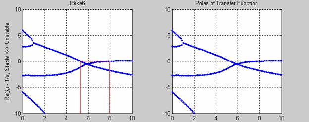
We can then use MATLAB’s pole-zero map function: [p, z] = pzmap(G)

Which, for the Schwinn Crown, has poles that look like this: a perfect match for the eigenvalues generated in JBike6

% From JBike6

% The linearized equations of motion read:

%

%       M0*qdd+(C1.*v)*qd+(K0+K2.*v^2)*q=0

%

% where v is the forward speed of the bike.

%

% Requires MATLAB’s Control System Toolbox

 

% set the bicycle parameters

JBini

 

% calculate the linearized equations of motion

JBmck

 

% calculate the weave and capsize speed

JBvcrit

 

% calculate the eigenvalues and eigenvectors for a speed range

JBeig

 

% plot only the Real part of the eigenvalues

subplot(1,2,1);

JBrev

title('JBike6'); a = axis;

drawnow;

 

% create transfer function from state-space representation

% use x1 = q1, x2 = q1_dot, x3 = q2, x4 = q2_dot

subplot(1,2,2);

v = 0:0.1:10;

M = inv(M0);

for i = 1: length(v)

    S = M*(C1.*v(i));

    K = M*(K0 + K2.*v(i)^2);

    A = -[0,      -1,     0,      0;

          K(1,1), S(1,1), K(1,2), S(1,2);

          0,      0,      0,      -1;

          K(2,1), S(2,1), K(2,2), S(2,2)];

     

    B = [0, 0,      0, 0;

         0, M(1,1), 0, M(1,2);

         0, 0,      0, 0;

         0, M(2,1), 0, M(2,2)];

    

    C = [1, 0, 0, 0];

    D = [0, 0, 0, 0];

    [numG, denG] = ss2tf(A, B, C, D, 2);

    G = tf(numG, denG);

    [p, z] = pzmap(G);

    plot(v(i).*ones(1, length(p)), p, '.'); hold on;

    %rlocus(G)

    %sisotool(G);

end

grid on; hold off; axis(a);

title('Poles of Transfer Function');